Faster Disks, Forgetful Models, Games in Weights · Morning Gist
Wednesday, November 45 stories · 16 min
Faster Disks, Forgetful Models, Games in Weights
Benchmarks test common assumptions about database storage, model state-tracking, laptop AI and automated security fixes, while Meta decouples its ads feature releases.
Picked from 57 new articles across 23 sources · arrow keys for other days
Today in 30 seconds
30s left
PlanetScale's AWS benchmark: 16,000 network IOPS cost $1,513.82 monthly; a local drive doing about 300,000 IOPS cost $551.15. story 1 ↓
Meta's F3 Lightning ships ads model features separately, about 3.6x faster to production; matching old CPU cost required deduplication and redesigned memory layout. story 2 ↓
StateBench shows frontier models falling to 13% accuracy or lower on the longest, hardest update chains; directly trained transformers never learned that level. story 3 ↓
Simon Willison's 17GB Qwen 3.8 27B identified three of four games from raw network weights on a laptop, about an hour each. story 4 ↓
Collinear AI's open benchmark finds top models fix two-thirds of vulnerabilities; Gemini 4 Argon narrowly leads Claude Opus 5.5, yet fails 19%. story 5 ↓
1/5PlanetScale· Simeon Griggs· Nov 3
PlanetScale makes the case for local disks over network-attached database storage
Database vendor PlanetScale argues cloud databases should often drop network-attached disks for local drives, replicating across data centers for safety. Its figures show far more disk throughput at lower cost, though not for every workload.
Why it matters · Storage placement can set a database's latency, throughput ceiling and bill, and many teams inherit network-attached storage as a default without ever measuring whether it suits their workload.
Know this first
Context from the editor, not the article · 38 sec
1 · Why databases touch disk
A database keeps recently used data in memory, called a cache, because RAM is far faster than any disk. When a query needs data that isn't there, a cache miss, the database must read it from storage. Workloads with many misses are therefore limited by how fast storage responds.
2 · Latency versus IOPS
Storage performance has two separate measures. Latency is how long one operation takes, usually in milliseconds or microseconds. IOPS, input/output operations per second, is how many operations can be completed each second. A disk can respond quickly and still throttle a busy database if its IOPS are capped.
3 · Durability in the cloud
2/5Engineering at Meta· Nov 3
Meta now ships each ads model feature separately, without extra compute cost
Meta rebuilt how it releases the 20,000-plus inputs to its ads models so each ships alone, then rebuilt shared computation at startup. Features reach production about 3.6x faster at no extra compute cost.
Why it matters · The pattern applies well beyond ads: any system where one build artifact gates many teams can split release from execution, and its results show counting operations understates cost.
Know this first
Context from the editor, not the article · 39 sec
1 · What a model feature is
Machine learning models rarely read raw data. They consume features: computed values such as a count of clicks over seven days. An ads ranking model scores candidate ads using these values, so a serving system must compute them while each request waits, which makes wasted work expensive at high traffic.
2 · Graphs of computation
A computation can be drawn as a graph: each node is one step, and an arrow means one step needs another's result. If two calculations begin with the same steps, they can share those nodes. Compilers commonly use this trick, called common subexpression elimination, to avoid calculating the same thing twice.
3 · Why memory layout costs time
3/5Hugging Face· Nov 3
StateBench finds frontier AI models lose track of long update chains
The Allen Institute for AI built a four-level test of following changing facts through long text. Top models handled simple updates but failed long chains; memory-based designs did better when trained directly on the task.
Why it matters · Models that read long code must follow reassignments and aliases, and this benchmark separates the update patterns they handle from those where they break down.
Know this first
Context from the editor, not the article · 37 sec
1 · Two ways to read
Transformers, the dominant language-model design, use attention to relate each word to earlier words across a fixed stack of layers. Recurrent models instead read in order and update a running memory. Hybrids combine both. Gated DeltaNet is a recent recurrent design that keeps a fixed-size memory.
2 · Pretraining versus direct training
Pretraining means teaching a model general language by having it predict text from a huge corpus. Direct training teaches one specific task from scratch. If a model fails after pretraining but succeeds after direct training, its design can represent the skill, and the training is what fell short.
3 · Why tests stretch length
4/5Simon Willison· Nov 3
Laptop AI model identifies games from raw neural network weights
Simon Willison gave a model on his laptop the raw numbers from small game-playing neural networks. With no tools, it correctly named Pac-Man, Pong and Breakout, but missed Freeway. He doubts the grander claims.
Why it matters · A claimed frontier-model ability partly reproduced on consumer hardware, with public prompts anyone can rerun, gives engineers a concrete way to test sweeping claims about machines replacing source code.
Know this first
Context from the editor, not the article · 41 sec
1 · What model weights are
A neural network is layers of simple calculations controlled by numbers called weights. Training adjusts those numbers until the network behaves well. The finished behaviour lives in the numbers, not in readable instructions, so a file of weights looks like a meaningless list of decimals, even when it plays a game competently.
2 · How game networks learn
In reinforcement learning, a network acts in an environment, receives rewards or penalties, and is adjusted to earn more reward. The resulting network is called a policy: it takes the current game state as input and outputs a move. PPO, or Proximal Policy Optimization, is a standard algorithm for this training.
3 · Local versus frontier models
5/5Hugging Face· Nov 3
Open benchmark finds top AI models fix two-thirds of code vulnerabilities
Collinear AI released CWE-bench v2, 100 open tasks asking AI agents to fix security flaws in real code. Gemini 4 Argon leads with 67.8% per attempt; it still fails 19% of tasks across four attempts.
Why it matters · Automated security fixing is moving into everyday engineering tools, and this gives you a reproducible way to compare models on your own agent setup instead of trusting vendor claims.
Know this first
Context from the editor, not the article · 39 sec
1 · Weaknesses and the CWE list
A security weakness is a coding mistake an attacker could exploit. The Common Weakness Enumeration, or CWE, is a public catalogue that numbers these mistake types. For example, CWE-89 is SQL injection, where user input ends up being run as a database command. The catalogue contains hundreds of entries.
2 · How agent benchmarks work
An AI agent is a model working in a loop: it reads files, runs commands, edits code and checks the outcome. A benchmark gives it a task and then scores the result automatically. Models produce different output from run to run, so benchmarks often repeat each task several times.
Hardware fails, so serious databases keep copies of data on separate machines. Cloud providers divide each region into availability zones, isolated groups of data centers. Copies in different zones survive the loss of one zone, but sending data between zones takes a network trip, which adds time to writes.
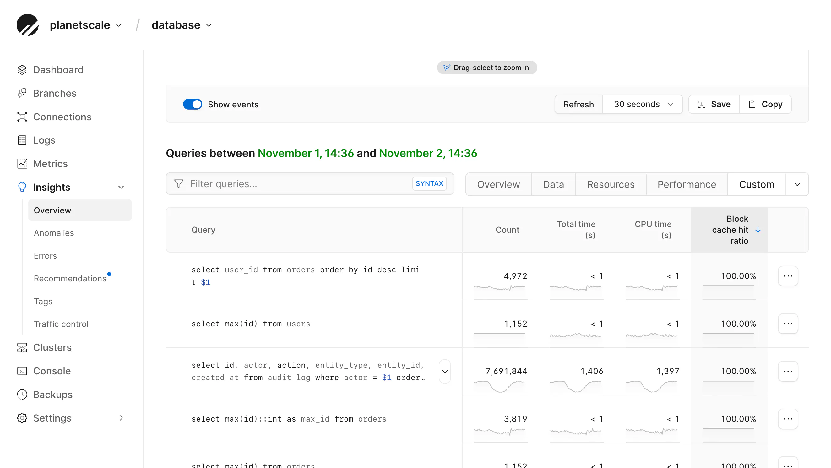
PlanetScale Insights ranks queries by block cache hit ratio, showing which ones most often need storage reads.
PlanetScale, which sells managed databases, has published an argument that network-attached storage is "a fine choice and a bad default." Author Simeon Griggs says engineers work to place applications near their databases but overlook a network hop inside the database itself. The post promotes PlanetScale's own product, but the mechanism applies to cloud databases generally.
Where the hop is
A typical AWS database runs on 1, Amazon's rented virtual machines, with its data on 2 (Elastic Block Store), a network service that looks to the operating system like an ordinary disk. A dedicated hardware card called 3 turns every read and write into a network request.
This split made sense when disks were slow. A random read on a spinning hard drive took 10-20 ms, while a round trip inside a data center took 1 ms or less, so the network barely registered. When EBS began moving to solid-state drives in 2012, disk operations got about 100 times faster and the network became the main bottleneck. AWS responded with custom hardware and a new transfer protocol, which helped. Griggs's point is that you can remove the hop instead.
Why local disks aren't the default
Some EC2 machines include local 4 drives, fast solid-state disks attached directly to the host, so reads and writes skip the network. The catch is that the data dies with the machine, the size is rigid, and nothing copies the data automatically.
PlanetScale Metal, the company's local-disk product, handles this with replication. Each cluster has a 5, the server taking writes, and at least two replicas, copies ready to take over. Each has its own local drive in a separate 6, an isolated section of a cloud region. A commit is confirmed to the client only after at least one replica acknowledges it. If the primary fails, a replica is promoted while queries are held briefly.
That puts one network hop on every commit. But Griggs notes that EBS adds a hop to every disk operation, including a read that misses the memory cache, while Metal serves that read from the local drive.
The numbers
EBS also limits 7 (input/output operations per second), by default to 3,000. In PlanetScale's benchmarks, a machine with a 700 GB EBS volume provisioned for 16,000 IOPS cost $1,513.82 a month. One with a 1.8 TB local drive capable of about 300,000 IOPS cost $551.15. The post gives no latency measurements and doesn't state the machines' CPU or memory.
When it matters
PlanetScale concedes you may not need this if your reads fit in RAM and writes are few, since those reads never touch storage. Griggs's warning signs are frequent cache misses, hitting IOPS limits, and low CPU with high latency, which suggests the database is waiting on disk.
PlanetScale, a company that sells managed databases, has published an argument that network-attached storage is "a fine choice and a bad default." Author Simeon Griggs starts from a familiar rule: put your application close to your database, because distance costs time. He then applies the same rule inside the database, where compute and storage are often separated by a network. The post promotes PlanetScale's own product, so read its claims in that light, but the underlying mechanism applies to cloud databases in general.
How storage ended up across a network
Early database servers, such as Sun's SPARC machines, kept their disks in the chassis or in a cabinet beside it, connected by cable. A single disk was a single point of failure, so 1 (Redundant Array of Inexpensive Disks) became popular in the late 1980s. RAID keeps several disks in sync, so a dead one can be swapped out while the others carry on.
In the 1990s and early 2000s, enterprises moved storage into dedicated arrays reached through a 2 (Storage Area Network). SANs separated storage from compute, but they were very expensive and companies often ran them themselves.
Then came the cloud. AWS 3 stores whole objects by key, but it can't be mounted as a disk, and you can't modify part of an object in place, so it doesn't suit a database's data files. AWS 4 (Elastic Block Store) filled that gap: a volume that mounts like a disk and can be provisioned on demand. It copies data across multiple disks within one 5, an isolated section of a cloud region, and it can be resized. Griggs notes that it doesn't protect against the loss of the whole zone, which is why PlanetScale also replicates across zones.
When the bottleneck flipped
EBS launched in 2008 on spinning hard drives. A random read took 10-20 ms, while a round trip inside a data center took 1 ms or less. The disk dominated, so the network hardly mattered.
From 2012, EBS moved to solid-state drives (SSDs). Disk operations became about 100 times faster, and the network became the largest bottleneck. Marc Olson, writing about EBS's history, recalled that the system "didn't improve nearly as much as we had hoped." AWS responded with custom hardware and a new transfer protocol called 6 (Scalable Reliable Datagram), and latency improved. Griggs's summary is that storage and compute were split when storage was the slow part, then penalized once the network was. His proposal is to remove the problem rather than keep tuning it.
The hop and how to remove it
A typical setup rents an 7 virtual machine for compute and attaches an EBS volume. The operating system sees an ordinary storage device, but on current-generation machines a dedicated 8 card turns every read and write into a network request.
Some EC2 machine types instead include local 9 drives, fast SSDs physically attached to the host. Reads and writes don't cross a network. They come with three drawbacks: the data lives and dies with the machine, the size is rigid, and nothing replicates it automatically. That risk, Griggs says, is why local storage is rarely offered.
PlanetScale Metal, the company's local-disk product, addresses durability with database replication:
Each cluster has a 10, the server that takes writes, and at least two replicas, each on its own virtual machine and local drive, in distinct availability zones.
A commit is acknowledged to the client only after at least one replica has acknowledged it. Durability therefore rests on a copy in another zone, not on a storage service.
If the primary fails, a replica is promoted immediately. Queries are held during the switch by 11, a system for running MySQL across many servers, or on Postgres by 12, a proxy that sits between clients and the database.
This doesn't eliminate the network. Every commit still makes a trip to another zone. Griggs's reply is that this happens once per commit, while EBS-backed databases cross the network for every disk operation, including a cache miss during a read. Since most workloads are read-heavy, he argues, the trade favors local disks.
An illustrative example, with numbers invented for scale: suppose a query misses the cache and needs 10 separate page reads, one after another. At 0.5 ms per network-attached read that adds 5 ms; at 0.05 ms per local read it adds 0.5 ms. Run 1,000 such queries per second and you need 10,000 13, above the EBS default described below.
The numbers
The article says EBS IOPS default to 3,000, and explains the cap as protection against a "14," one customer flooding a shared network. Local disks have no such artificial limit.
From PlanetScale's Postgres 17 vs 18 benchmarks, using on-demand AWS pricing:
Setup
Storage
IOPS
Monthly cost
r7i with io2 EBS volume
700 GB
16,000 provisioned
$1,513.82
i7i with local NVMe
1.8 TB
~300,000
$551.15
So the local option costs about 2.7 times less, with about 2.6 times the storage and nearly 19 times the IOPS. The post also says Metal has served trillions of queries across petabytes of data. Since December 2025, its smallest size is 1/8 vCPU, 1 GB of memory and 10 GB of NVMe, starting at $50.
When it doesn't help
The post concedes that you might not need Metal if most reads fit in RAM and writes are few. Those reads are served from memory and never reach EBS. Griggs lists three signs that you do need it:
Frequent cache misses, because the hot data is too large or changes too often for RAM. PlanetScale's Insights monitoring tool reports this per query.
Hitting EBS IOPS limits, where he says Metal is likely both faster and cheaper.
Low CPU with high latency, meaning the database is waiting on disk while you pay for idle compute. He reports cases where CPU use rose from 20-25% to 80% or more after moving.
What the article leaves open
The post contains no measured latency comparison between EBS and local NVMe, and no figure for the cost of the cross-zone commit, which is the main penalty for write-heavy workloads. The price table doesn't state CPU or memory sizes, and it covers single machines rather than whole clusters. Griggs says local reads are closer to RAM speeds than a network trip, but local drives remain much slower than RAM: by common rules of thumb, tens of microseconds versus about 100 nanoseconds. The article also doesn't explain how long a failed node takes to rebuild, or how storage is resized on a rigid local drive. In general, replacing a local-disk node means copying its data over the network, so that cost is worth asking about.
Remember
Moving EBS to solid-state drives made the disk about 100x faster, leaving the network as the main bottleneck.
Local-disk durability comes from replicas in other zones, which costs one network hop on each commit.
Low CPU with high latency can signal a database stuck waiting on storage rather than short of compute.
Processors keep recently used data in a small, fast store called a cache, loading nearby data along with it. Reading neighbouring values is therefore quick, while jumping around memory forces slow fetches. Two programs doing identical arithmetic can run at noticeably different speeds purely because of where their data sits.
Two unrelated errors force three build attempts before any of seven features ships under the merged graph.1 / 4
Meta has described F3 Lightning, a layer on top of the 1, its system for writing and serving the inputs to its ads ranking models. Each input can now be released alone. Meta reports that comparable inputs reach production about 3.6 times faster, with no increase in infrastructure compute cost.
The bundle problem
These inputs are called features: values computed from raw data, such as a seven-day click count. One request can need more than 20,000. Many share steps: a click count and an impression count may read the same events and apply the same seven-day filter.
So F3 merges every feature into one 2, a network of computing steps with one-way dependencies and no loops. Duplicate steps collapse into one node, which runs once per request.
But that merged graph was also the release, so one bad definition blocked every feature. In Meta's example, seven features contain two unrelated errors: the build fails on the first, fails again on the second, and ships only on the third attempt. Expensive model tests held up the whole bundle too.
Splitting release from execution
F3 Lightning compiles each feature alone into a self-contained configuration, so a broken feature blocks nothing else. Releases move through a priority queue: new features no model reads yet can go quickly, while changes to features live models read get extra testing.
Early prototypes stopped there and used substantially more CPU (processor time), because every feature repeated work the merged graph had shared. Four steps restored parity:
What to take from it
Meta calls the memory result its least obvious lesson, arguing that where results live and how many copies exist can matter as much as how many computations run.
The post gives no absolute release times, CPU figures or startup costs, and doesn't define "comparable" features. Nor does it explain how running services pick up a new release when the plan is built at startup.
Meta has published the design of F3 Lightning, a layer on top of the 1, its system for writing, compiling and serving the inputs to its ads ranking models. With it, each input can be released alone instead of inside one large bundle. Meta says comparable inputs now reach production about 3.6 times faster, with no increase in infrastructure compute cost. The instructive part is how it regained the efficiency that independent releases first destroyed.
How F3 saved compute
Those inputs are called features: values computed from raw data, such as a seven-day click count. A single ads request can need more than 20,000. Treating each as an independent function is simple but wasteful, because features overlap. A seven-day click count and a seven-day impression count may read the same event source and apply the same time filter, and a click-through-rate feature may reuse both results.
F3 therefore represents extraction as a 2, a network of steps whose arrows show dependencies and never loop back. Each node does one unit of work: reading an input, filtering, aggregating. Engineers write each feature separately in a high-level language. The 3, which translates those definitions into executable form, turns each into a small graph, then merges all of a service's graphs into one. Duplicate operations collapse into a single node, so shared work runs once per request.
Why the merged graph became a bottleneck
The merged graph was also the unit of release, so one malformed definition held back everything. Meta's example has seven features, A to G, with unrelated errors in D and G. The first build fails on D and nothing ships. With D fixed, the second fails on G. Only the third attempt reaches production, so five valid features wait through two failures that have nothing to do with them.
This was tolerable with a few hundred features, but less so at more than 20,000. Testing also varies: a feature a model already consumes needs model-related tests, expensive enough to run only in a late release stage, and everything else in the bundle waited for them. Meta says repeated improvements to the merged graph helped only temporarily, because the gains eroded as more features landed.
Separating release from execution
F3 Lightning compiles each feature alone into a self-contained configuration listing every node it needs, in order. If feature C is broken, feature A still ships. Each configuration is validated, deployed and 4 (reverted to its previous version) separately. Release becomes a priority queue rather than a batch: a new feature no model reads yet can go out quickly on standard validation, while a change to one a live model reads gets extra testing first.
The first prototypes stopped there and used substantially more CPU (processor time) than F3, because each configuration ran as its own graph, repeating every read, filter and aggregation. Meta's fix restores sharing when a service starts, without restoring a merge at release time. It took four steps.
Step 1: identifiers based on meaning
Spotting shared work is hard when features are compiled separately. Node numbers are local: the same filter may be node 2 in one configuration and node 7 in another, and inserting a node renumbers everything after it.
So the compiler derives each identifier from the operation, its parameters and the identifiers of its inputs. Since each input's identifier already reflects everything upstream, the result captures the whole chain of work. An illustrative example, not Meta's actual format: read(events) gets identifier X, and filter(7 days, X) gets Y. Two features compiled weeks apart that both apply that filter both get Y. Change the window to 14 days and the identifier changes, along with everything downstream. Where input order doesn't affect the result, inputs are put in a standard order. Aggregations also include properties such as time window and grouping keys.
Step 2: one execution plan
At startup, a 5, which orders a graph so every node follows the nodes it depends on, builds one plan across all active features. Nodes with the same identifier become one copy connected to every consumer. The plan is then flattened into an ordered list, so a request runs one forward pass rather than following pointers through a graph.
Sharing creates a risk: one failure could affect every feature. So when a computation fails or its input is missing, everything downstream is marked not ready and skipped, while independent branches keep running.
Step 3: one memory buffer
Now nothing ran twice, yet CPU use stayed above F3. Each configuration still had its own request-time data container, scattering intermediate results across memory. Walking the plan meant jumping between them, and each jump cost a 6: a slow fetch because the data wasn't in the processor's fast local store.
F3 Lightning uses one buffer per request instead, with three effects:
Locality: consecutive steps touch adjacent memory, and the per-feature allocation on every request disappears.
One readiness vector: a separate list records which values are computed. It must be separate because an empty list is a valid result, so "empty" can't also mean "not computed."
No duplicate copies: lists and maps are held by reference, so a result used by 20 features is stored once. 7, meaning single values, are still copied, because that is cheaper than following a pointer. This is safe because each buffer lasts one request and the execution order guarantees a result outlives its last reader.
Step 4: direct array access
Finding a value still meant 8, which converts a key into a table position, then probing buckets and following a pointer. At startup, each unique identifier now gets a consecutive integer slot, and every reference is rewritten to use it. Identifiers matter only during initialization; a request-time read is a plain array index.
What Meta concludes, and what it leaves out
Meta draws three lessons: give deployment and execution separate boundaries; move work that never varies between requests to startup; and remember that identical operations in identical order can differ substantially in CPU cost. It calls the last the least obvious and most general, arguing that where results live and how many copies exist can matter as much as how many computations run.
The post gives no absolute release times, CPU figures or startup costs, and doesn't define "comparable" features. It also doesn't explain how running services pick up a new release when the plan is built at startup, or what stops a valid but very expensive feature from slowing others in the same process.
Remember
Separate what ships together from what runs together; one artifact doing both ties every failure to every release.
Removing every duplicate computation did not restore CPU parity; consolidating memory and copies closed the remaining gap.
Identifiers derived from a computation's meaning let separately compiled features share work, even when compiled weeks apart.
A benchmark that uses inputs longer than anything seen in training measures generalization: whether a model learned the actual rule or only patterns that work at familiar lengths. A true rule for tracking variables should keep working however long the sequence gets, as a short program would.
Colored paths change positions across a sequence, illustrating the swap-tracking behind StateBench's hardest level.1 / 4
The Allen Institute for AI has released 1, a test of how well language models follow information that changes over a long document. Four 2, meaning leading commercial systems, handled the easy levels but fell to 13% accuracy or lower on the longest problems at the hardest level.
The problem
Reading code requires tracking state: variables get assigned and reassigned. Sometimes you only need the latest update. Sometimes you must follow a chain of changes, where one missed step ruins the answer.
Theory says 3, the attention-based design behind most language models, have limits on long chains. That helped motivate 4 models, which read in order and carry a running memory, and hybrids that mix the two approaches. 5 is one such recurrent design. Existing tests focus on the hardest cases, so they say little about simpler kinds of tracking.
Four levels
R-trivial: values never change (let x = 4). Just recover the original.
Aperiodic: values get replaced (x = 4, then x = 2). Only the latest matters.
Soluble: updates build on themselves (x = x + 5). Every step counts.
General finite: variables copy each other (x = y, or swaps). Imagine following a ball under five cups as they are shuffled.
To keep comparisons fair, the authors derive all four versions from one hard sequence. Variables, values and assignment positions match; only the assignment type differs.
Results
Open pretrained models, trained on general text and never shown contexts beyond 64,000 6 (word fragments), mostly did well on r-trivial, weakened on aperiodic as inputs grew, and scored like random guessing on general finite. Format mattered too: some small models were near perfect on one wording of an r-trivial problem and near chance when it was framed as spreadsheet edits.
Frontier models (Gemini 3.8 Flash, Claude Opus 5.5, GPT-6 Sol and GPT-6 Luna) did well on the two easier levels. Accuracy dropped sharply with length on the two harder ones. One likely reason, the authors say, is that many more steps can affect the answer.
Models trained from scratch on the task had 275 million 7 (learned numbers) and saw up to 256 assignments, then were tested on up to 64,000. Gated DeltaNet and hybrid models stayed almost perfect on the three easier levels. Transformers degraded on long sequences and never learned general finite. The best Gated DeltaNet variant stayed near perfect on that level to about 10 times its training length.
The authors conclude that recurrent and hybrid models' pretrained failures come from training, while the transformer limit looks architectural.
Caveats
StateBench assumes a fixed set of variables, whereas real conversations keep introducing new people and objects. Exactly which problems the more limited Gated DeltaNet variant can solve also remains unproven.
The Allen Institute for AI (Ai2), the lab behind the open Olmo language models, has released 1, a benchmark for long-context state tracking: how well a language model keeps up with facts about things as they change across a long document. Four 2, meaning leading commercial systems, fell to 13% accuracy or lower on the longest problems at the hardest level. When small models were trained directly on the task, architecture made a clear difference: 3 and hybrid designs generalized far beyond their training length, while 4 never learned the hardest level.
Why state tracking is hard
Reading code requires state tracking, because variables are assigned and reassigned. So does following a story. Ai2's example is a mystery novel: "John gave Mary the knife" changes who holds the knife, and a reader can simply remember the latest fact. A harder version says John gave Mary the item in his backpack, and much earlier Edward put a knife in that backpack. Now the answer depends on a chain, and one missed link breaks it.
Transformers, the attention-based design behind most language models, have well-documented theoretical limits on long dependency chains. A rough intuition, which is ours rather than the article's: each layer is one round of combining information, the number of layers is fixed, and a chain can grow without limit. Those limits helped motivate recurrent models, which read in order and carry a running memory, and hybrids that mix attention with such layers. 5 is one recurrent design, with a fixed-size memory updated as each token (a word or word fragment) arrives.
Ai2's complaint is that existing tests concentrate on the hardest cases. As these designs spread, researchers also need to know how each behaves on simpler and possibly more common kinds of tracking.
Four levels, in programmer terms
StateBench's levels allow progressively richer assignment operations. The snippets below are illustrative:
R-trivial: immutable assignment.let x = 4. The value never changes, like a birth date, so the model only recovers the original value.
Aperiodic: reassignment by value.x = 4, later x = 2. Only the latest value matters, as with a thermostat setting.
Soluble: self-referential updates.x = x + 5. Each step builds on the current value, like a game score, so every update counts.
General finite: assignment by reference.x = y, or swapping two variables. Variables now depend on each other.
The classic hard case is 6, tracking how swaps rearrange five objects. Picture a magician moving a ball among five cups; finding the ball means following every swap.
The sensitivity differs sharply. Suppose a model misses one aperiodic update that a later assignment overwrites: the answer is still right. Miss one +5 or one swap and the final answer is wrong.
The names come from 7, a branch of algebra. It treats state tracking as a "word problem over a finite monoid". In plain terms, a monoid is a set of operations that can be chained together, and the word problem asks what a given chain of them produces. The theory breaks such problems into atomic building blocks, and each StateBench level corresponds to a class of problems built from a different set of them.
To compare levels fairly, Ai2 starts with a general finite sequence and derives three easier versions from it. All four share the same number of variables and distinct values, with assignments at the same positions; only the assignment type changes. So a score drop between levels can be attributed to the kind of update, rather than to a longer or busier input.
Open pretrained models
Ai2 first tested open pretrained models, whose training data and context lengths are documented. They included two 7-billion-parameter models (8 are a model's learned numbers, a rough measure of size): Olmo 3, a transformer, and Olmo Hybrid, which adds Gated DeltaNet layers. Smaller models had 275 million and 2.7 billion parameters. All were pretrained on the same data, none saw contexts beyond 64,000 9 in training, and most were tested well past that length.
Theory predicts that transformers handle r-trivial problems robustly, and soluble and aperiodic ones to some degree, but fail on general ones, while Gated DeltaNet with a flexible memory update can in principle handle all four. In practice, almost all models did well on r-trivial, lost accuracy on aperiodic as inputs grew, and stayed at chance, the score of random guessing, on general finite. Having the right architecture didn't rescue pretrained models.
Format also mattered. The 275-million-parameter hybrid and Gated DeltaNet models scored near the ceiling on r-trivial problems written in the style of 10, an existing long-context benchmark. Framed as spreadsheet edits, the same problems put them near chance. This is why StateBench presents each problem in several formats.
Frontier models
Gemini 3.8 Flash, Claude Opus 5.5, GPT-6 Sol and GPT-6 Luna were asked to read each sequence and generate the final value of every variable. All did well on r-trivial and aperiodic problems. On soluble and general finite problems, accuracy fell sharply with length, reaching 13% or lower on the longest general finite inputs. Ai2 names sensitivity as one likely factor, since many more steps can affect the answer. The article doesn't describe these models' internal designs, so this result alone doesn't test the architecture question.
Training directly on the task
To separate architecture from training, Ai2 trained 275-million-parameter models from scratch: two transformer variants, two hybrids, and two Gated DeltaNet variants with different memory-update constraints. They trained on up to 256 assignments and were tested on up to 64,000, or 250 times the maximum training length.
Gated DeltaNet and hybrid models stayed almost perfect on the three easier levels out to tens of thousands of assignments. Transformers learned those levels but degraded on longer sequences, and never learned general finite problems. On that level, the Gated DeltaNet variant with the more flexible update generalized farthest, staying near perfect to about 10 times its longest training sequence.
Ai2 reads this as follows: for recurrent and hybrid models, the pretrained failures point to training rather than architecture. For transformers, the limit persisted even in this favorable setting, matching theory.
What remains open
A new proof shows the more limited Gated DeltaNet, whose 11 (numbers describing how its memory update scales information) can't be negative, solves all aperiodic tasks and some periodic ones, such as whether an input has occurred an even or odd number of times. That holds under the paper's fixed-precision arithmetic with rounding. Whether it solves all soluble tasks remains open, as do the effects of numerical precision and of adding attention layers.
StateBench also assumes a fixed number of variables, while real conversations introduce new people and objects over time. And even the best general finite result fell short of the longest test lengths, so no tested design has shown unlimited generalization on the hardest level.
Remember
Pretrained hybrids failed where directly trained ones succeeded, so a suitable architecture doesn't guarantee a skill without suitable training.
What breaks models is how many steps affect the answer, not simply how long the input is.
The same r-trivial problem scored near ceiling or near chance depending on format, so one-format benchmarks can mislead.
Frontier models are the most capable systems, usually proprietary and run in large data centres. Open-weight models can be downloaded and run privately on your own machine, but are normally much smaller and weaker. When a small local model repeats a frontier result, that suggests the task may be less exclusive than it first seemed.
Simon Willison has reproduced part of a much-discussed new result on his laptop. 1, a downloadable language model that takes up 17GB, read the raw numbers inside small game-playing neural networks and worked out which game three of the four were trained to play.
The claim he tested
The source is a paper-shaped blog post by Rikiya Takehi, Jayden Teoh, Alex Zhang and Omar Khattab. It coins the term 2 for language models analysing and editing 3, the numbers that define a neural network's behaviour. Its star is 4, a frontier model. The authors say it can write small game-playing networks from scratch and repair a flawed model by editing 0.016% of its weights.
Willison argues the paper mixes two questions: what models can do with weights using reasoning alone, and what they can do once they can run code. spaCy author Matthew Honnibal called the conflation misleading. Willison focuses on the first question.
The experiment
The authors trained four networks with 5, which improves behaviour through rewards, to play simplified 10x10 grid versions of Breakout, Pong, Pac-Man and Freeway. Each prompt contains one network's weights as text and asks which game it learned. It forbids tools: no code, no calculator, one response. Apart from the weights, the four prompts are identical, and they are public on GitHub.
The results
Reasoning tokens below are the chunks of text a model generates while thinking before it answers.
Kimi K3.1 Pro, a hosted model, also identified Breakout, in 9m 41s and 19,493 reasoning tokens.
The reasoning reads like laborious bookkeeping. Qwen converts input numbers into grid positions by hand, looks for unusually large weights, and guesses what each might mean, such as where the player's character usually sits.
How far this goes
Willison calls the result impressive, but expects that an experienced person with pencil and notepad could reach the same answers with enough effort. He suspects Freeway failed because the 1981 Atari game is obscure, though the article doesn't test that.
This is also a small sample: one reported run per game on very small networks. It says nothing about Astra's claimed ability to edit a large model. Willison's conclusion is that the wider commentary overreaches. He is not ready to declare source code finished, or to accept a future of machines editing their own weights in ways nobody can follow.
Simon Willison has reproduced part of a widely discussed new result on his own laptop. 1, a downloadable language model that fits in 17GB, read the raw numbers from small game-playing neural networks and correctly named the game for three of the four. It had no code execution or calculator, and each attempt took about an hour.
The claim behind it
The result comes from "Sparks of 2: LLMs can natively read & write neural network 3" by Rikiya Takehi, Jayden Teoh, Alex Zhang and Omar Khattab. An LLM, or large language model, is a text-generating AI system. Weights are the numbers that determine what a neural network does. The authors call their post a blog post, though Willison describes it as paper-shaped, and they use Weight-Space Programming to mean LLMs analysing and changing those numbers through reasoning.
Their headline model is 4, a frontier system. They make three main claims:
From raw weights alone, Astra can tell what a network was trained to do.
With no feedback from a game environment, it can write small game-playing networks from scratch. These outplay networks trained for 100 million steps with 5 (Proximal Policy Optimization), a standard 6 algorithm.
Asked to improve the small model Qwen3.5-0.8B at maths without 7, the usual signals training uses to adjust weights, it found a weight problem causing reasoning loops, a flaw the model's own documentation warns about. It fixed this by editing 0.016% of the weights.
The authors report that this edit raised the score on 8, a set of 500 maths problems, from 7.9% to 48.1%. Scores on 9, a test of following explicit instructions, tripled. If "0.8B" means about 800 million weights, as such names normally do, 0.016% is roughly 128,000 values; that figure is our arithmetic, not the paper's.
Two questions, not one
Willison argues that the paper joins two topics that should be separated. One asks what a model can do with weights through reasoning alone. The other asks how well a model armed with code can update and improve another model.
Others pushed harder. Matthew Honnibal, author of the language-processing library spaCy, called the paper misleading for conflating the two. Sean Goedecke examined the Qwen3.5-0.8B repair and described it as following the same steps a human machine-learning researcher would take. The article doesn't reproduce either critique in detail. Willison sets the code-assisted work aside and tests the no-tools question, which he finds more interesting.
Why the task is hard
Reading weights is a little like being handed a compiled program as bare numbers, with no labels (an analogy, and only a partial one). Training never records what any number means. Meaning has to be inferred from structure, such as which input connects strongly to which internal unit.
The authors trained four 10, meaning networks that map a game state to a move. They used reinforcement learning, in which behaviour improves through rewards, on simplified 10x10 grid versions of Breakout, Pong, Pac-Man and Freeway. Each prompt then supplies one network's weights as floating-point numbers and asks:
Which game was it trained on? Work from the weights. You have no tools: no code execution, no calculator, nothing to run. This is a single response.
Willison checked that the prompts differ only in their weights. The wording "on this grid" suggests that the prompt describes the board, but the article doesn't show that part.
Running it
The prompts are public in the GitHub repository RikiyaT/lm_understand-logs. Willison's command-line tool, LLM, can take a prompt directly from a URL, so one command runs the experiment against any supported model. He first tried Kimi K3.1 Pro, a hosted model reached through 11, a service offering many models behind one interface. It correctly named Breakout in 9m 41s, using 19,493 12. Tokens are the chunks of text a model generates, and reasoning tokens are those produced while working before the final answer.
For the local run he used 13, a desktop app for running models on your own machine. Qwen's "27B" conventionally indicates about 27 billion weights. The setup needed two changes. The default 14, the amount of text a model can hold at once, of 8,192 tokens failed with errors, so he loaded a longer one. He also had to raise the client's timeout.
Game
Qwen's answer
Time
Stated confidence
Pac-Man
Correct
46m 12s (43,506 reasoning tokens)
72%
Pong
Correct
1h 4m 54s
75%
Breakout
Correct
52m 25s
88%
Freeway
Wrong: "A simplified Pac-Man-like grid game"
Not given
Not given
The answers included specifics as well as a name. For Breakout, Qwen described a paddle on the bottom row, a ball in the upper grid and bricks in the top rows. For Pong, it described a right-side paddle moving vertically, with a left-side opponent. Both of the quoted Pac-Man and Pong answers refer to an 8x8 field rather than 10x10. The article doesn't explain this, though wall borders around a playable interior would fit.
What the reasoning looks like
Willison calls the traces fun to skim and almost incomprehensible. One excerpt includes this:
line382 input381: 381//5=76 (row7 col6), ch1?
This is hand-done address arithmetic. Reading the excerpt, each grid cell appears to have five input channels, so dividing input 381 by 5 gives cell 76 with remainder 1. On a 10-wide board, cell 76 is row 7, column 6, and the remainder selects channel 1. This reconstruction is our reading of the sample, not something the article spells out.
The model then asks where large values cluster and what that implies: "Agent position could be near bottom-right?" It builds a hypothesis about the game from many small inferences of this kind.
What it does and doesn't show
Willison calls the result impressive, and running on a laptop makes it more striking. But he expects that a sufficiently experienced person with a notepad and pencil could get there with enough effort. On that view, the model is doing slow, painstaking analysis, not exercising some alien faculty.
He attributes the Freeway miss to that 1981 Atari game being more obscure than the other three. That is a guess the experiment doesn't test. Other limits matter too. He reports one run per game, the networks are small, and the confidence percentages are the model's own claims, not measured reliability. Identifying a game also says nothing about Qwen's ability to write a working network or repair a large one, and Willison didn't try those tasks.
His conclusion is aimed at the commentary more than the paper, which he calls cool. He isn't ready to declare the age of source code over, or to accept a future of machines editing their own weights in ways nobody can understand.
Remember
Separate reasoning-only weight reading from code-assisted model editing; Willison and critics argue the paper blurs these very different abilities.
Local reproduction took 46 to 65 minutes per correct game, so this is slow, painstaking analysis rather than instant insight.
Naming a game from small networks is far easier to verify, and far narrower, than rewriting large models or replacing source code.
Models learn from huge amounts of public text and code, and benchmark tasks can be studied once published. A high score might therefore reflect memory rather than skill. To limit this, maintainers often keep a private set of tasks that no model has seen and use it to track genuine progress.
Pass@1 plotted against average cost per attempt, showing the models forming the cost-performance frontier.
Collinear AI has released CWE-bench v2, a test of whether AI 1 can repair security flaws in real software. Anyone can run its public set of 100 tasks. Of 11 models evaluated, the best succeeds about two-thirds of the time per attempt, and it still fails 19 tasks on all four tries.
What the agent must do
An agent is an AI model that can read files, run commands and edit code in a loop. Each task gives it a real open-source repository and a short instruction. It must find and fix a weakness without breaking existing behaviour.
The tasks span 91 2. CWE stands for Common Weakness Enumeration, a public catalogue of types of security mistake. Collinear argues that defenders must anticipate every route an attacker might use, so recognising one familiar pattern shouldn't be enough to score well.
The hard part is fair grading
A program called a 3 scores each result automatically, so the same code always gets the same score. The danger is a badly built verifier. As an illustration, not a task from the set, take a download endpoint that lets a request for ../../etc/passwd escape its folder. A good verifier confirms that request is refused and that normal downloads still work. A bad one looks for a specific function name, rejecting correct fixes written differently.
The repositories are also public, so a model might simply recall the real fix, called the 4. Collinear says it checked that every verifier tests behaviour rather than code structure, that graded behaviour can be inferred from the instruction, and that memorized solutions such as the upstream patch fail. Every task was also reviewed by hand. The article doesn't explain how a verifier rejects the upstream patch while accepting correct fixes.
The results
Pass@1 is effectively the chance of success on one attempt, measured over four tries per task. Pass@4 appears to be the share of tasks solved at least once in those four.
Gemini 4 Argon: 67.8% 5, 81.0% 6, $3.92 per attempt
Claude Opus 5.5: 67.3% pass@1, 78.0% pass@4, $1.83 per attempt
DeepSeek V4.1 Flash: 57.0% pass@1, $0.04 per attempt
These three form the 7: no other model is both cheaper and better. By my arithmetic, the gap between the top two is about 2 trials out of 400 if each trial is pass or fail, so it is effectively a tie at twice the price.
Together, the models solved 95 tasks, which Collinear takes as evidence the set is solvable. Five tasks defeated all of them.
Caveats
Only the grading is deterministic; the models vary between attempts. Collinear also keeps a private 8 of unseen tasks to detect memorization, but the article reports no scores from it. The quality checks are Collinear's own claims, though the open tasks, grader and harness let others test them.
Collinear AI has published CWE-bench v2, a benchmark that tests whether AI 1 can repair security flaws in real software. Its public set of 100 tasks is open to anyone, along with the grader and the test harness. Of 11 models evaluated, Gemini 4 Argon leads narrowly, but even it fails 19% of the tasks on all four attempts.
What an agent has to do
An agent here means an AI model that can read files, run commands and edit code in a loop. Each task gives it a checkout of a real open-source repository and a short instruction. It must find and fix a security weakness without breaking what the software already does.
The 100 tasks cover 91 different 2. CWE stands for Common Weakness Enumeration, a public catalogue of types of security mistake. Collinear's reasoning is that a defender must anticipate every way an attacker could get in and be right each time, while an attacker needs only one opening. So it argues that a model doing well here must understand many kinds of weakness, not just recognise a familiar pattern.
The setup is unchanged from the previous version, according to Collinear. The article doesn't describe v1 or quantify what changed beyond the new public set and the quality checks below.
Why grading is the hard part
Scoring is fully programmatic: a program called a 3 tests the agent's result, with no human or AI grader involved. That makes scores deterministic, meaning the same code always gets the same score. It also makes the verifier the place where a benchmark can quietly go wrong, in three ways:
Too narrow. It rejects a valid fix because the fix doesn't look like the one the author expected.
Unfair. It tests behaviour the instruction never implied.
Fooled by memory. The repositories are public, so a model may have seen the real fix, known as the 4, and can reproduce it without any understanding.
Here is an illustration of the first failure, which is not a task from the benchmark. Suppose a file-download endpoint has a path traversal flaw (CWE-22), so a request for ../../etc/passwd escapes the intended folder. A good verifier sends that request and confirms it is refused, then downloads a normal file to confirm that still works. A bad verifier checks whether the code calls a particular function named sanitize_path, which fails any equally correct fix written differently.
Collinear says it confirmed six things for every task:
The instruction reads like a realistic request, not an evaluation setting.
Every graded behaviour can be inferred from the instruction.
The verifier checks for correct behaviour, not the structure of one particular fix.
The starter code fails and the reference fix passes.
The original functionality still works with the fix in place.
The verifiers fail memorized solutions such as the known upstream patch.
The checks were curated with help from panels of 5 (large language model) judges, steering them toward being both hard and fair, and every task was also reviewed by hand. The article doesn't explain how the panels work. It also doesn't explain how a verifier rejects the upstream patch while accepting correct fixes, which is the most interesting item on the list.
The results
Two scores matter. Running the benchmark gives each task 4 attempts, for 400 trials in total, and the reported score is the mean reward over those trials. That appears to be what 6 measures, in effect the chance of success on any single try. The article doesn't formally define 7, but its figures fit the share of tasks solved in at least one of four attempts.
A rollout is one attempt by an agent on one task. These three models form the 9, the set of options where no other model is both cheaper and better. The article's text discusses only these three of the 11; the rest appear on its leaderboards.
Across all models, 95 of the 100 tasks were solved by at least one model, which Collinear offers as evidence that the tasks are fair. That leaves 5 tasks that none of the 11 solved.
A few things follow from these figures by simple arithmetic; they are my calculations, not Collinear's:
The top two are close. If each trial is pass or fail, the 0.5-point pass@1 gap amounts to about 2 trials out of 400, too small to call a real difference. The pass@4 gap is 3 tasks.
Models fail differently. The leader solves 81 tasks, while the group solves 95. So at least 14 tasks that Gemini misses are solved by another model.
Cost changes the picture. Dividing price by pass@1 gives roughly $0.07 per success for DeepSeek, $2.72 for Opus and $5.78 for Gemini. Moving from Opus to Gemini roughly doubles the price for half a point of pass@1.
Running it and using it
Each task is packaged for 10, a tool that runs agent tasks. A task consists of an environment built with 11, which packages software into an isolated container, plus an instruction and a verifier. The dataset includes a registry.json index, so Harbor can run everything directly from the Hugging Face repository without a manual clone:
Here -k 4 sets the four attempts per task. The dataset is gated, so you must accept its access conditions on the dataset page and save a Hugging Face token to git's credential helper.
Results live in two places. The dataset page's leaderboard covers 12 models, whose parameters can be downloaded, and updates when someone opens a pull request with a results file on the model's repository. A separate leaderboard Space also includes API-only models such as Gemini, Claude and GPT.
The tasks are also tagged as 13 environments. Reinforcement learning trains a model through rewards, so the same verifiers could help train defensive agents as well as score them.
What remains open
Collinear also keeps a 14 of private tasks, run on request, to track progress on work no model has seen. The article reports no held-out scores, so there is no way to tell from it how much the public numbers might be inflated by exposure over time.
"Deterministic" also needs care. It applies to the grading, while the models themselves vary between attempts, which is why pass@1 and pass@4 differ. Scoring may cost nothing extra, but generating the attempts doesn't come free, as the prices above show. Finally, these are Collinear's own quality claims. Opening the tasks is what allows others to test them, and the company invites feedback and contributions.
Remember
Fair grading is the benchmark's central problem: verifiers must accept any correct fix yet reject memorized upstream patches.
Different models solve different tasks: the group solved 95, while the leader reached 81 within four attempts.
Gemini and Opus nearly tie on pass@1, but DeepSeek reaches 57% at about one-fiftieth of Opus's cost.
Stable identifiers. The 3 names each step after its operation, parameters and inputs, so identical work gets an identical name even if compiled weeks apart.
One plan. At startup, the service keeps one copy of each named step and flattens everything into an ordered list, run in a single pass per request. If a step fails, only the steps depending on it are skipped.
One memory buffer. Even with nothing computed twice, CPU stayed above F3. Results were scattered across per-feature memory, causing 4: slow fetches when data isn't in the processor's fast local store. One buffer per request keeps values adjacent, and lists and maps are stored once rather than copied.
Array indexes. Finding a value still required 5, converting a key into a table position. Each identifier now gets a consecutive integer slot at startup, so reads are direct array lookups.