Deficits, Nobels and 130 Million Missing People · Morning Gist
Thursday, October 155 stories · 16 min
Deficits, Nobels and 130 Million Missing People
Today: why surging AI imports didn't widen the trade deficit, a Nobel for central banks' core model, weak housing demand, and doubts about China's population count.
Picked from 33 new articles across 16 sources · arrow keys for other days
Today in 30 seconds
30s left
A New York Fed economist finds that government borrowing, not the surge in AI imports, explains almost all of the wider U.S. trade deficit since before the pandemic. story 1 ↓
Hall and Woodford won the economics Nobel. Hall showed that huge forecasting models failed, and Woodford built the three-equation model central banks now use. story 2 ↓
With mortgage rates near 7.5%, purchase applications are down 16% from a year ago. Listings are up 4.8% but still below 2019 levels. story 3 ↓
Demographer Yi Fuxian uses vaccine and school data to argue China has about 1.27 billion people, not 1.4 billion, which would change its per-person and pension numbers. story 4 ↓
Liaquat Ahamed tells Tyler Cowen that two decades of falling prices after 1873 left growth intact but did lasting political damage. story 5 ↓
Consumer prices rose 3.7% over the year to September, and Social Security has announced next year's cost-of-living increase.
1/5Liberty Street Economics (NY Fed)· Julian di Giovanni· Oct 14
AI imports surged, but the U.S. trade deficit didn't widen because of them
AI equipment made up 23% of U.S. imports in 2025. A New York Fed economist finds the AI boom hasn't widened the deficit with the rest of the world. Bigger government deficits explain nearly all of the change.
Why it matters · The piece shows why a flood of imports doesn't mean a wider deficit. It also points to the variables that could change that if AI spending keeps accelerating.
Know this first
Context from the editor, not the article · 29 sec
1 · What the current account is
The current account is the broadest measure of a country's balance with the rest of the world: mainly trade in goods and services, plus income flows. The U.S. has run a current account deficit for decades, meaning it buys more abroad than it sells.
2 · Saving minus investment
A basic national-accounting identity says the current account equals national saving minus domestic investment. A country whose investment exceeds its own saving must borrow the difference from abroad, and that borrowing shows up as a deficit.
3 · Three kinds of saver
National saving is the sum of household, business and government saving. A government deficit counts as negative saving. So larger budget deficits lower national saving, just as households spending more would.
2/5Conversable Economist· conversableeconomist· Oct 14
Hall and Woodford win economics Nobel for the model central banks use
Robert Hall and Michael Woodford won the 2026 economics Nobel. Hall showed that old-style economic models failed to predict consumer spending. Woodford built the New Keynesian model that central banks now use to set interest rates.
Why it matters · When the Federal Reserve explains a rate decision by pointing to "inflation expectations," it is reasoning inside the framework these two economists built.
Know this first
Context from the editor, not the article · 30 sec
1 · Micro versus macro
Microeconomics studies individual households, firms and markets. Macroeconomics studies whole economies: total output, unemployment, inflation and interest rates. The split took hold after the Great Depression showed that an entire economy could fail at once.
2 · Stabilization policy
Stabilization policy is how governments try to smooth booms and busts. The central bank sets interest rates (monetary policy), and the government sets taxes and spending (fiscal policy). The goal is steady growth, low unemployment and stable inflation.
3 · The Phillips curve
The Phillips curve is a pattern seen in the decades after the Second World War. Low unemployment tended to come with rising inflation, and high unemployment with falling inflation. Policymakers treated it as a menu of trade-offs they could choose from.
3/5Calculated Risk· CalculatedRisk by Bill McBride· Oct 14
Mortgage rates near 7.5% weaken home buying as listings slowly rise
The 30-year mortgage rate hit 7.5%, its highest since November 2023. Weekly data show fewer purchase loan applications and slightly more homes for sale. Bill McBride expects existing-home sales to slow and prices to face pressure.
Why it matters · If you plan to buy, sell or refinance, these weekly numbers show how fast higher rates are changing buyer demand and housing supply, months before official sales and price data.
Know this first
Context from the editor, not the article · 31 sec
1 · Why weekly housing data
Official home sales and price reports come out with a lag of one to several months. Mortgage application surveys and listing counts come out every week, so analysts use them as early signs of where sales and prices are heading.
2 · The rate lock-in effect
Many owners hold mortgages taken out at low rates before 2022. When new rates are much higher, moving means giving up a cheap loan. That keeps many people from listing their homes, which has held inventory below normal levels.
3 · How rates affect payments
On a 30-year fixed loan, a small change in the rate makes a big difference to the monthly payment. That is why higher rates cut how much house buyers can afford, and why refinancing stops making sense when rates rise.
4/5Marginal Revolution· Tyler Cowen· Oct 14
Demographer argues China has 130 million fewer people than reported
University of Wisconsin demographer Yi Fuxian says China inflated its numbers. He compares official birth counts with vaccine supplies and school records and puts the population near 1.27 billion, not the official 1.4 billion.
Why it matters · Population is the denominator behind China's per-person income, its labor-force projections and its pension maths. A 9% error would change how investors and policymakers read the world's second-largest economy.
Know this first
Context from the editor, not the article · 30 sec
1 · China's population debate
China officially reports about 1.4 billion people. Births have fallen for years, and the population began shrinking in 2022. Some outside demographers have long argued the official totals are too high, especially for births since the 1990s.
2 · How births get counted
China builds population figures from censuses held every ten years, household registration (hukou), hospital records and school enrollment. These sources should broadly agree. Gaps between them are the usual way demographers test whether the official numbers hold up.
3 · BCG vaccine
5/5Marginal Revolution· Tyler Cowen· Oct 15
Liaquat Ahamed on why the 1873 crisis hurt politics more than growth
Economist Tyler Cowen interviewed historian Liaquat Ahamed about his new book, 1873. Ahamed argues that the deflation after 1873 did little harm to growth because wages could fall. The bigger damage was political.
Why it matters · It helps separate two questions people usually lump together: whether a financial shock shrinks the economy, and who ends up paying for it.
Know this first
Context from the editor, not the article · 27 sec
1 · The Panic of 1873
A financial crash that began in Vienna in May 1873 and spread to New York that September. It started roughly two decades of falling prices, which historians often call the Long Depression.
2 · Gold versus bimetallism
Under bimetallism, a currency is backed by both gold and silver. In the 1870s, Germany and then other countries moved to gold alone. Demand for gold rose and the world's money supply grew more slowly, which pushed prices down.
3 · Ahamed's earlier book
Lords of Finance (2009) follows the central bankers of the 1920s. Ahamed blames their attachment to gold for helping cause the Great Depression. The book won the 2010 Pulitzer Prize for History.
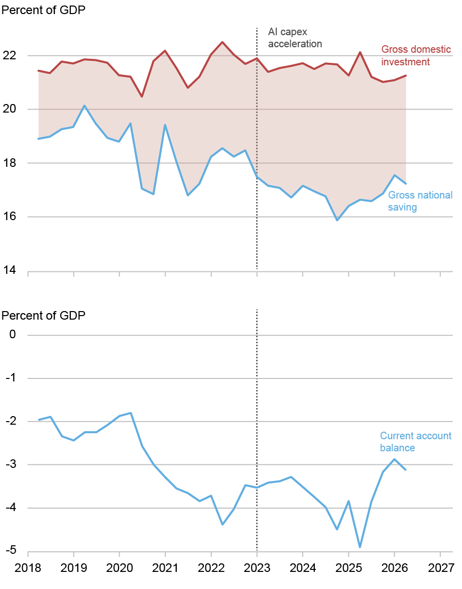
Investment stayed flat as a share of GDP after 2018, while saving fell and the current account deficit widened.1 / 2
AI-related goods such as chips, servers and computing equipment made up 23% of U.S. imports in 2025, according to research cited in a new New York Fed post. Yet Julian di Giovanni, a research advisor at the New York Fed, finds the AI boom has done essentially nothing to the U.S. 1, the broad balance of trade and income with the rest of the world.
Why imports don't set the deficit
The current account is a net measure. It equals national saving minus domestic investment. A country can import lots of equipment without a wider deficit if it saves enough at home to pay for the investment. The deficit grows only if total investment rises faster than saving, or saving falls.
The deficit has grown, from about 2.2% of GDP in 2015–19 to about 3.7% since 2023. Di Giovanni traces where that came from.
Investment: reshuffled, not raised
Total investment averaged 21.3% of GDP before the pandemic and 21.5% from 2023 to early 2026, when AI capital spending took off. The data-center surge was offset by fading factory construction after the 2022 industrial-policy laws, soft non-tech investment and falling housing investment.
Private saving: holding up
In the dot-com boom of 1995–2000, private saving fell nearly 3 points of GDP as households spent their stock gains. Today it is 20.8% versus 21.3% before the pandemic, a gap partly explained by households running down pandemic savings.
Business saving is the cash firms keep after expenses, excluding investment. It is also steady: 10.9% of GDP recently, against about 10.5% before the pandemic and a dot-com low of 8.8%. Di Giovanni argues the key difference is who is investing. In 2000 it was young, cash-poor telecom firms whose saving collapsed. Today it is the most cash-rich companies in the economy, funding 2 largely from their own earnings.
Government: the real driver
3 fell from about −2.2% of GDP to about −4.0%, the opposite of the dot-com era, when tax windfalls produced a 4% surplus. Measured from late 2019, the saving–investment gap widened about 2.4 points: roughly 1.75 from government borrowing, 0.5 from lower private saving and about zero from investment.
The caveat
Big tech's announced capex for 2026–27 is considerably larger than what has been built so far, and the drags on other investment won't last. If they fade while AI spending rises and starts to eat into corporate cash, the deficit would widen through both higher investment and lower 4. The post doesn't estimate how much.
The puzzle
Imports of semiconductors, servers and computing equipment have climbed steeply during the AI boom. Recent research cited by Julian di Giovanni, an economist at the Federal Reserve Bank of New York, puts AI-related goods at 23% of all U.S. imports in 2025. You might expect that to drag the U.S. 1 (the broad balance of trade and income with the rest of the world) further into deficit.
In a Liberty Street Economics post, di Giovanni argues that it hasn't. The deficit did widen, from about 2.2% of GDP on average in 2015–19 to about 3.7% since 2023. But the AI buildout explains essentially none of that change. Most of it came from government borrowing.
Why imports alone don't set the deficit
The key is that the current account is a net measure. By national-accounting identity it equals gross national saving minus gross domestic investment. A country can import huge amounts of capital equipment and still keep its external balance steady, as long as it saves enough at home to pay for that investment.
Here is an illustration with made-up numbers. Suppose a country saves 18% of GDP and invests 21%. It has to borrow the 3-point gap from abroad, so its current account deficit is 3% of GDP. Now suppose AI spending lifts investment in data centers by 1 point while investment in factories and housing falls by 1 point. Total investment stays at 21%. The country might import more chips and fewer other goods, but the gap, and therefore the deficit, stays the same. The deficit widens only if total investment rises without a matching rise in saving, or if saving falls.
So di Giovanni asks three questions: did total investment rise, did private saving fall, and did government saving fall?
Investment was reshuffled, not increased
Gross domestic investment averaged 21.3% of GDP in the five years before the pandemic. It averaged 21.5% over 2023 to early 2026, when AI 2 ("3") accelerated, and 21.1% over the latest four quarters. In di Giovanni's words, the AI boom "is not visible in the aggregate investment rate at all."
The reason is offsetting weakness elsewhere. AI's share of nonresidential investment has been rising. But the factory-construction surge that followed the 2022 industrial-policy laws (the CHIPS Act and the Inflation Reduction Act, though the post doesn't name them) has faded. Spending on structures and equipment outside the tech sector has been soft, and residential investment has been declining. Data centers and information-processing equipment filled the gap without pushing total investment up relative to saving.
Households aren't spending their stock gains
The obvious comparison is the dot-com era. Between 1995 and 2000, private saving fell by nearly 3 percentage points of GDP as households spent out of rising stock wealth, which economists call a 4. Nothing like that is happening now. Private saving has averaged 20.8% of GDP since 2023, against 21.3% before the pandemic. Di Giovanni attributes that half-point gap as much to households running down their pandemic-era savings as to anything AI-related.
Who is doing the investing matters
Business saving is revenue minus expenses, excluding investment spending. Roughly, it is the cash firms keep. Here the two booms differ most. The dot-com buildout was led by young telecom and equipment firms with thin or negative operating cash flow. When their profits shrank late in the boom and dividends stayed sticky, retained earnings and 5 fell just as investment peaked.
The AI buildout is led by some of the most cash-generating firms in the economy. Business saving has averaged 10.9% of GDP over the past four quarters, close to the roughly 10.5% before the pandemic and well above the dot-com low of about 8.8% in late 2000 and early 2001. These firms are paying for their capex largely out of their own cash, so the spending doesn't drain national saving.
Government moved the other way
6 is where the two episodes differ most sharply. In the dot-com years it rose by nearly 5 points of GDP, from a deficit of about 1% in 1995 to a surplus of about 4% in 2000, as capital-gains taxes poured in. That windfall offset much of the household 7, which is one reason the current account widened by "only" about 2.5 points back then.
Today the government is pulling saving down. Government saving fell from about −2.2% of GDP in 2015–19 to about −4.0% since 2023, a drop of roughly 1.75 points.
The decomposition
Measured against the end of 2019, the saving–investment gap has widened by about 2.4 percentage points:
Government dissaving: about 1.75 points
Lower private saving: about 0.5 points
Higher investment: essentially zero
Di Giovanni concludes that fiscal policy has been the main driver of the current account, private saving has played a smaller part, and there is "no discernible investment channel." One quibble: the 2.4-point figure uses the end of 2019 as its baseline, while the 2.2%-to-3.7% comparison uses 2015–19 averages. The post doesn't reconcile the two, so the precise sizes depend on the baseline chosen.
What could change
The author flags an important caveat. The big tech firms' announced capex plans for 2026 and 2027 are considerably larger than what they have already built. Meanwhile, the slump in housing and non-tech investment won't last forever. If those drags fade while AI spending speeds up, total investment would finally rise. If the spending also starts to eat into the firms' cash, business saving would fall. Both would widen the deficit, which would be a dot-com-style pattern arriving late.
The post doesn't estimate how large that effect could be or when it might happen. It also doesn't model the import side directly, for example how much of future AI capex will go to imported versus domestically made equipment. Its contribution is a framework and a reading of the data so far: the AI boom has not yet been big enough, relative to the rest of the economy, to move the U.S. external balance.
Remember
Since late 2019, government borrowing explains about 1.75 of the 2.4-point widening in the saving–investment gap.
AI investment displaced weaker spending on factories and housing, so total investment stayed near 21% of GDP.
Cash-rich tech firms funding AI from earnings kept business saving steady, unlike the cash-poor dot-com builders.
Robert E. Hall and Michael Woodford have won the 2026 Nobel memorial prize in economics "for microeconomic foundations of macroeconomic stabilisation." Timothy Taylor of the Conversable Economist blog explains the phrase by tracing how the way economists model whole economies has changed.
The 1,000-equation era
After the Great Depression, economists learned to measure entire economies. Simon Kuznets invented what became 1, and Wassily Leontief mapped which inputs go into which outputs. Add computers, and you get huge forecasting models. Lawrence Klein's Wharton model grew from 200 equations to more than 1,000. Each equation estimated a stable link between broad totals, such as how much spending follows a given amount of income.
The 1970s broke that confidence. High unemployment and high inflation arrived together ("2"). The models said this couldn't happen, because they relied on the 3, which held that high unemployment pulls inflation down.
Hall: spending should look random
Consumption is about two-thirds of total demand. The old models assumed people spend a fixed share of each extra dollar of income, estimated from past behaviour. In a 1978 paper, Hall argued that people instead decide how much to spend by looking ahead: how safe their job seems, and whether recession or inflation is coming.
If spending already reflects people's expectations, it changes only when those expectations change. That happens only with news, which by definition can't be forecast. So changes in spending should be a "4," where the best guess for next period is this period. When Hall tested this, the giant models forecast consumption no better than that simple rule.
Taylor calls this a "hammer-blow." The old models were snapshots with no actual households, firms or central bank making decisions, so they couldn't show behaviour shifting when policy shifted.
Woodford: a compact replacement
Later work produced many insights but, in Taylor's view, no simple core model. Woodford built one: the 5, set out in his 2003 monograph. Its simplest version has three equations:
Households: Hall's forward-looking spending.
Firms: price-setting when changing prices is costly.
Central bank: an interest-rate rule.
Two frictions give policy a job. Firms have some market power and charge markups over cost, and prices and wages are "6," meaning they adjust slowly. Even with people reacting to policy, well-timed interest-rate and budget decisions can steady the economy. Central banks and finance ministries now run larger versions fitted to their own economies.
The gaps
Taylor calls extending the model "very much a work in progress." For example, the basic version has no financial sector, so banks and credit play no role in it.
The 2026 Nobel memorial prize in economics went to Robert E. Hall and Michael Woodford "for microeconomic foundations of macroeconomic stabilisation." Timothy Taylor, who writes the Conversable Economist blog and is managing editor of the Journal of Economic Perspectives, explains what that phrase means by retelling how macroeconomics has been done over the past 50 years. He admits he is painting with "an industrial-power spray-gun" rather than a fine brush.
The old way: the economy as a giant spreadsheet
The word "macroeconomics" grew out of the Great Depression. In 1933 the Norwegian economist Ragnar Frisch separated "micro-dynamic" analysis of one part of the economy from "macrodynamic" analysis of the whole system. Measurement came next. Simon Kuznets invented what became gross domestic product (1), the total value of goods and services an economy produces, and won the Nobel in 1971. Wassily Leontief built the input-output method, which treats the economy as a huge table showing which inputs go into which outputs. He won in 1973.
Combine those tables with computers and you get forecasting models. Lawrence Klein's Wharton model began in the late 1960s with 200 equations and grew past 1,000, and Klein won the Nobel in 1980. Each equation estimated a stable relationship between broad totals, such as how much spending follows from a given amount of income, using past data. The hope was to forecast booms and busts and to design policy that would prevent another Depression.
For a while in the 1960s that hope looked justified. Then the 1970s brought deep recessions alongside high inflation. This combination, called "2," could not happen in the big models, because they were built on the 3: high unemployment was supposed to pull inflation down.
Hall's challenge: spending should look random
Most critics wanted to repair the big models. Hall's 1978 paper questioned the whole approach, and Taylor explains it through consumption, which makes up about two-thirds of total demand.
The 1960s models treated spending as a function of current or recent income. People had a "4": a fixed share of each extra dollar of income that they spend rather than save. That share was estimated from the past. Hall argued instead that people decide how much to spend by looking ahead: how secure their job seems, and whether a recession or inflation is coming.
That idea produces a test. If today's spending already reflects everything people expect about the future, spending changes only when those expectations change. Expectations change only in response to news, and nobody can forecast news. If you could, it would already be part of your expectations. So month-to-month changes in consumption should be unpredictable: a "5," in which the best forecast of next period is simply this period.
An illustration with made-up numbers: if a household spends $4,000 this month, the random-walk forecast for next month is $4,000. Knowing last year's income pattern adds nothing. Hall compared the big models' consumption forecasts with this naive rule, and the 1,000-equation models did no better.
Taylor calls this, together with related work by others, "a hammer-blow" to old-style macro. The models were snapshots of relationships between totals. They contained no consumers, firms or central bank actually making decisions, so they had no way to show behaviour changing when policy or expectations changed. A new framework took shape over the 1970s and 1980s and brought Nobels to Robert Lucas (1995), Finn Kydland and Edward Prescott (2004), and Edmund Phelps (2006). Taylor's view is that it offered many separate insights but no compact core model to build on.
Woodford's synthesis: the 6
Woodford supplied that core, building on Hall's consumption theory. The result is the New Keynesian model, which Woodford summarized and extended in his 2003 monograph. The Nobel committee's background paper lists what the new framework had to do:
Accept, as Keynes did, that markets can fail and that government intervention can help.
Treat economy-wide outcomes as the sum of decisions by individual households and firms, not as fixed links between totals.
Model people as forward-looking: they watch where monetary and fiscal policy are heading and react to it.
Allow recessions to have different causes, which may call for different policy responses.
Two "frictions" give policy something to fix. First, competition is imperfect, so firms charge 7, the cost of producing one more unit. Second, prices and wages are "8": changing them is costly, so they adjust slowly and resources go unused in the meantime. The committee notes that even though households and firms in the model adapt to policy changes, well-used monetary and fiscal policy can still raise welfare by steadying the economy after shocks.
Firms: how profit-maximizing firms set prices when changing them is costly. This is a new, expectations-based version of the Phillips curve.
Central bank: an interest-rate rule.
The model was first meant for monetary policy and later became the main tool for fiscal policy too. Central banks run medium- and large-scale versions fitted to their own economies, and finance ministries build their own variants.
What remains open
Taylor sums up the shift this way: 1960s macro assumed that relationships between totals stay roughly constant over time. It had no consumers, firms or policymakers forming expectations, no imperfect competition and no sticky prices. In short, it lacked microeconomic foundations. He calls the work of extending Woodford's basic model "very much a work in progress." His example is that the three-equation version has no financial sector, a notable gap given how much recent recessions have involved banks and credit. The article does not explain how central banks have added finance to the model, or how well the New Keynesian model has forecast recent inflation. For those debates, Taylor points readers to the Nobel committee's "Scientific Background" paper and to Jordi Galí's 2018 Journal of Economic Perspectives article "The State of New Keynesian Economics: A Partial Assessment."
Remember
A model with 1,000 equations forecast consumer spending no better than assuming next period equals this one.
Modern central bank models start from decisions made by forward-looking households and firms, not from fixed links between economy-wide totals.
The basic New Keynesian model has no financial sector, a gap economists are still working to fill.
MBA purchase index, weekly and four-week average: applications to buy homes remain at depressed levels.1 / 3
The average 30-year fixed mortgage rate reached 7.5% in the week ending October 9, 2026. That is the highest since November 2023 and more than a percentage point above a year earlier. Two weekly data series collected by Bill McBride of Calculated Risk show buyers pulling back while homes slowly build up on the market.
Fewer people applying to buy
The 1, the trade group for mortgage lenders, surveys loan applications every week. Its 2, which counts applications to buy a home, fell 4% in the week and was 16% below the same week last year. Applications overall fell 2.7% after adjusting for normal seasonal patterns.
Here is an illustrative example of what a point of interest means. On a $400,000 loan, the monthly payment rises from about $2,530 at 6.5% to about $2,800 at 7.5%. That is roughly $270 more each month for the same house.
Refinancing has almost stopped
The 3 was 56% lower than a year earlier. Refinancing only pays off when you can switch to a lower rate. With rates up a point, few recent borrowers can. MBA economist Joel Kan said last week's drop came mostly from a 5% fall in 4 refinances, which are loans backed by the Federal Housing Administration and popular with first-time buyers.
Borrowers are also turning to 5. These carry a lower rate for the first few years and then reset to market rates. ARMs made up 10.5% of applications, the highest share since October 2025. A rising ARM share usually means buyers are stretching to afford a monthly payment.
More homes for sale
6 tracks active single-family listings each week. Inventory was up 4.8% from a year ago and down 5.1% from the same week in 2019, the last normal year before the pandemic. Supply is growing but is still a little below pre-pandemic levels, and the gap is shrinking.
What it means
McBride argues that rising inventory plus weak demand means existing-home sales will probably slow over the coming months and prices will come "under pressure". He does not predict outright price declines. The post doesn't explain why rates rose, break the data down by region, or put a size on the price effect. Applications also miss cash buyers, so read them as a direction, not an exact count.
Bill McBride of the Calculated Risk newsletter has pulled together two weekly data series. Both point the same way: higher mortgage rates are reducing housing demand while supply slowly grows. Mortgage applications fell again in the week ending October 9, 2026. The number of single-family homes listed for sale kept rising compared with a year earlier.
What happened to rates
The 1, the industry group for mortgage lenders, runs a weekly survey of loan applications. In the latest survey, the average 30-year fixed rate was 7.5%. That is the highest since November 2023 and more than a percentage point above the rate a year ago.
Here is an illustrative calculation, not from the article, to show what a point means. On a $400,000 loan, the monthly principal and interest is about $2,530 at 6.5% and about $2,800 at 7.5%. That is roughly $270 more every month for the same house. Buyers can either pay more, buy something cheaper, or wait.
Demand: purchase applications
The MBA's Market Composite Index measures the overall number of mortgage applications. It fell 2.7% from the week before after 2, which removes normal calendar patterns such as the autumn slowdown. Without that adjustment it fell 2%.
The 3 tracks applications to buy a home, as opposed to refinancing an existing loan. It fell 4% in the week on both an adjusted and an unadjusted basis. It was 16% lower than in the same week a year earlier. McBride describes purchase activity as "depressed", and his chart (weekly figures plus a four-week average) shows applications stuck at low levels.
Refinancing has nearly stopped
The 4 slipped 0.4% in the week but was 56% lower than a year earlier. The reason is simple. People refinance when they can swap their current rate for a lower one. With rates a point higher than last year, almost nobody who borrowed recently gains anything by refinancing. McBride's long-term chart, going back to 1990, shows refinance activity near historic lows. According to MBA economist Joel Kan, much of last week's decline came from a 5% drop in refinance applications for 5 loans. These are loans insured by the Federal Housing Administration and are popular with first-time and lower-down-payment borrowers.
Borrowers move toward adjustable-rate loans
Kan says borrowers are relying more on 6 to keep payments down. An ARM charges a lower fixed rate for an introductory period, often five or seven years, and then resets in line with market rates. ARMs made up 10.5% of applications, the highest share since October 2025. A rising ARM share is a common sign of affordability strain. Borrowers accept the risk of higher payments later in return for a lower payment now.
Supply: inventory edging up
For supply, McBride uses data from 7, which tracks active listings of single-family homes each week. As of October 9:
Inventory was up 4.8% from the same week of 2025, compared with up 4.4% the week before.
Inventory was down 5.1% from the same week of 2019, compared with down 5.5% the week before.
The 2019 comparison matters because 2019 was the last "normal" market before the pandemic and before the jump in rates that froze many owners in place. Supply is growing compared with last year but is still a little below pre-pandemic levels, and the gap is narrowing week by week. The Altos chart shows the usual seasonal pattern since 2015: inventory rises through summer and falls into winter. The 2026 line sits just under the 2019 line.
McBride's reading
McBride argues that the two series together show inventory picking up slightly while demand is weak. With 30-year rates close to 7.5%, he expects existing-home sales to slow over the next few months and house prices to come under pressure. He is careful with that word. He does not forecast falling prices, only pressure on them.
What the article doesn't cover
The post is a short data note, so several questions remain open:
Why rates rose. The article does not say what pushed mortgage rates to 7.5%, whether Treasury yields, inflation data or something else.
Regional differences. The inventory figures are national. In past cycles, some local markets saw supply rise much faster than others, but the post does not break this down.
How much "pressure". No size or timing is given for any price effect. And because inventory is still below 2019, sellers are not yet facing a flood of competing listings.
Limits of application data. Applications are not completed purchases. Some buyers apply more than once, and cash buyers do not show up at all. The data are best read as a direction, not an exact count.
The short version: the cost of borrowing has risen, fewer people are trying to buy, almost no one is refinancing, and homes are slowly piling up on the market. Each of those has historically come before slower sales.
Remember
Refinance applications are 56% below a year ago because almost no recent borrower can lower their rate.
Adjustable-rate loans hit 10.5% of applications, a sign buyers are stretching to afford monthly payments.
Listings are up 4.8% from 2025 but still 5.1% below 2019, so supply is recovering without a glut.
BCG is a tuberculosis vaccine. China gives it to every newborn within a day of birth, so the amount of vaccine used should roughly track the number of births. It usually comes in multi-dose vials that spoil soon after opening.
Image: Marginal Revolution
Yi Fuxian, a University of Wisconsin-Madison demographer and longtime critic of China's population policies, argues in a new 1 that China's population may be about 1.27 billion, not the official 1.4 billion. The gap of up to 130 million people is roughly the population of Mexico. The Wall Street Journal reported the claim, and economist Tyler Cowen passed it on at Marginal Revolution under the title "China fact (?) of the day". The question mark signals his own uncertainty.
How he checks the numbers
No one outside China can count its people directly. So Yi compares sources that ought to agree: census results, school enrollments, hospital births, vaccine batches and household registrations. He says the errors run the same way across many of them, pointing to systematic inflation. Two examples:
Vaccine vials. Every newborn in China must get a 2 tuberculosis vaccine within 24 hours of birth. BCG comes in multi-dose vials that must be thrown away 30 minutes after opening. Few babies are ready in the same half-hour, so Yi says each vial yields only about 1.2 to 1.6 doses in practice. From 2018 to 2020 the government approved about 5.8 million vials a year, but officially reported more than 14 million births a year. Those figures only fit if each vial vaccinated about 2.4 babies, which Yi calls impossible nationwide.
A shrinking birth year. Officials reported 17.7 million births in 2000. The 2010 census counted only about 14.4 million ten-year-olds. About 14.2 million finished middle school in 2015. That leaves roughly 3.5 million children from one year unaccounted for. Very few children die or emigrate before age 10, which makes the original count look too high.
Why it matters
Yi argues the inflated figures have fed overconfidence in Beijing and anxiety in Washington. The article doesn't go into the economics, but they are simple arithmetic. Fewer people means higher GDP per person. It also means a smaller future workforce and a heavier pension burden than official projections assume.
Reasons for caution
The vaccine test depends on Yi's doses-per-vial assumption and on vial approvals covering all the vaccine supply. The excerpt doesn't show how he tested either.
Statistical agencies sometimes adjust birth counts upward to make up for births that went unregistered, which was common under the one-child policy. Whether China's adjustments were too large is the real question, and the article doesn't settle it.
This is one long-standing critic's analysis, with no response quoted from officials or other demographers.
Yi Fuxian is a demographer at the University of Wisconsin-Madison and a longtime critic of China's population policies. In a new 1, reported by the Wall Street Journal and picked up by economist Tyler Cowen on Marginal Revolution, he argues that China's real population may be about 1.27 billion, not the 1.4 billion officially reported. The difference, up to 130 million people, is about the population of Mexico and roughly 9% of the official total.
Cowen titled his post "China fact (?) of the day". The question mark tells you how much he vouches for the claim: he is passing it on, not endorsing it.
Why the number is hard to check
No outsider can count China's people directly. Figures come from a census every ten years, from household registration (the 2 system that ties people to a home district), from hospital birth records and from school enrollment. Each source has its own blind spots and its own incentives. Local officials may gain from reporting more residents, for example, and parents may have hidden births during the one-child era. So demographers test the totals by checking one source against another. Yi says that is what he did, comparing censuses, school enrollments, hospital births, vaccine batches and household registrations. He reports that the errors run the same way across many of these sources: the numbers are systematically too high.
The Marginal Revolution excerpt gives two of his tests.
Test 1: counting vaccine vials
China requires every newborn to get a 3 tuberculosis vaccine within 24 hours of birth. That makes vaccine use a rough stand-in for births. Yi's argument goes like this:
BCG comes in multi-dose vials, and an opened vial must be thrown away after 30 minutes.
Few hospitals have several newborns ready for vaccination within the same half-hour. In practice, Yi says, each vial yields only about 1.2 to 1.6 usable doses.
From 2018 to 2020 the government approved about 5.8 million vials a year.
On Yi's figures, 5.8 million vials × 1.2–1.6 doses works out to about 7 to 9.3 million babies vaccinated a year. (That multiplication is ours, not the article's.)
Official statistics reported more than 14 million births a year over the same period.
To square the official births with the vial supply, each vial would have to cover about 2.4 babies. Yi calls that medically and practically impossible across a whole country.
Test 2: following one birth year through school
The second test follows the same group of children over time. The 4 reported 17.7 million births in 2000. When those children were 10, the 2010 census counted about 14.4 million. When they finished middle school in 2015, about 14.2 million graduated. Roughly 3.5 million children, about one in five of the reported 5, are missing.
Few children die between ages 0 and 10 in a middle-income country, and emigration at those ages is small. A gap that large is hard to explain unless the original birth count was too high. One detail favors Yi: the cohort hardly shrinks between age 10 and 15. That suggests the shortfall is built into the starting figure rather than caused by children dropping out or leaving later.
What it would mean
Yi argues the distortion has warped strategic thinking on both sides of the Pacific. It feeds overconfidence in Beijing about China's size and staying power, and anxiety in Washington about the same. The article does not spell out the economic consequences, but they follow from basic arithmetic. If there are fewer people, the same GDP means higher income per person. It would also mean a smaller future workforce, faster ageing and a heavier pension burden than official projections show.
Caveats
The excerpt leaves several obvious objections unanswered:
Vial assumptions. The vaccine test depends on the 1.2–1.6 doses-per-vial figure and on approvals capturing all the supply. If some vaccine came in different vial sizes, came through other channels, or was used more efficiently in big urban maternity wards, the gap narrows. The excerpt doesn't say how Yi handled these possibilities.
How the 2000 figure was built. As a general practice, statistical agencies adjust raw counts upward when they think births went unreported. During the one-child era, hiding births was a real problem. Whether the 17.7 million figure includes that kind of adjustment, and whether the adjustment was justified, is the heart of the dispute. The article doesn't go into it.
The source. Yi has argued for many years that China overstates its population. That doesn't make him wrong, but this is one researcher's analysis, not a consensus estimate. The excerpt includes no response from Chinese officials or other demographers.
What remains open is whether these independent checks hold up when other demographers look at them, and whether the 130 million figure is a firm estimate or the top of a range. Yi's own phrasing, "as much as", suggests the latter.
Remember
Using Yi's own dose figures, 5.8 million vials a year could vaccinate only about 7–9 million newborns, not the 14 million reported.
About a fifth of the 17.7 million births reported for 2000 never appear in later census or school counts.
A smaller population would mean higher GDP per person and a weaker workforce and pension outlook than official numbers suggest.
Tyler Cowen, an economist and the author of the Marginal Revolution blog, has posted his podcast interview with Liaquat Ahamed. Ahamed is a former investment manager and the author of Lords of Finance, a Pulitzer-winning history of the central bankers behind the Great Depression. His new book is 1873. The post itself is only a short teaser, but the excerpts deal with a real question: why do some financial crises do lasting damage while others don't?
Two crashes, two outcomes
Cowen points out the tension himself. Lords of Finance convinced him that crises matter. 1873 almost convinced him they don't, because the world kept growing. After the 1, a crash that spread from Vienna to New York, prices fell for about two decades. Yet by one measure Cowen cites, the major economies still grew about 2.5% a year.
Ahamed says the book is really about the 2 that followed, and that a better title would have been The First Great Deflation.
Why falling prices didn't cause a slump
Deflation is usually dangerous because nominal wages are "3": the pay figure on a contract is hard to cut. If prices fall 3% but pay can't, each worker effectively costs 3% more, and firms lay people off instead. That pattern helped make the 1930s so severe.
After 1873, Ahamed says, things were different "because prices were flexible. Nominal wages went down." The economy adjusted through lower pay rather than mass unemployment.
Where the cost showed up
Ahamed argues the real damage was in who won and who lost, and in the politics that followed. The excerpt doesn't spell out the mechanism. The standard one is that falling prices make existing debts heavier, which hurts farmers and other borrowers and helps lenders. He links the period to US populism, a return of protectionism in Europe, a "retreat from liberal ideas," and Britain's 1882 invasion of Egypt.
According to the episode summary, the two also discuss Bismarck's role in ending 4. Bimetallism means backing money with both gold and silver. When Germany switched to gold alone, other countries followed, and the scramble for gold pushed world prices down. Other topics include Britain's 1926 return to gold and lessons from the 5 on Ireland and Pakistan. The post lists these without explaining them.
The takeaway, and the limits
The main lesson is that how much a crisis hurts depends on how the economy adjusts afterwards. Flexible wages turned the shock into a political fight over losses rather than lost output. The teaser doesn't explain why wages were more flexible then, or how the growth figure was measured. For those answers you'll need the full transcript or the book.
Tyler Cowen, an economist at George Mason University, has published an episode of his interview podcast, Conversations with Tyler, with Liaquat Ahamed. Ahamed is a former investment manager and World Bank official and the author of Lords of Finance, a history of the central bankers whose policies helped bring on the Great Depression. His new book is called 1873. Cowen's blog post on Marginal Revolution includes only a few excerpts, but they raise a useful question: when does a financial crisis actually do lasting damage?
The puzzle Cowen starts with
Cowen says the first book convinced him that financial crises matter a great deal. The second, he says, nearly convinced him they don't, "because the world just keeps on growing." Both books cover a global financial crash, but the aftermaths were very different. After 1929 the world fell into the Great Depression. After the 1, a crash that began in Vienna and spread to New York, the world entered a long stretch of falling prices but kept growing. By one measure Cowen cites, the major economies grew about 2.5% a year for the 20 years after 1873.
Ahamed's answer is that 1873 is mainly about what happened after the crash, not the crash itself. He says a better title would have been The First Great Deflation. The crisis set off "a sequence of effects throughout the world which damaged the political economy of the world for the next 20 years."
Why 2 didn't wreck growth this time
Economists usually treat deflation as dangerous because nominal wages are "3": employers find it hard to cut the pay figure written into a worker's contract. Here is an illustrative example. Prices fall 3% in a year, but wages can't be cut. The real cost of each worker then rises about 3%, so firms lay people off instead of paying less. That was a big part of what made the 1930s so severe.
Ahamed says the 1870s and 1880s were different "because prices were flexible. Nominal wages went down." When wages could fall along with prices, the economy adjusted through lower pay rather than mass unemployment. Output kept rising.
Where the damage went instead
Ahamed argues that "the distributional consequences and the political impact of those distributional consequences were much more damaging than the pure economic consequences." The excerpt doesn't spell out the mechanism. The standard one is that falling prices raise the real value of debts. A farmer who borrowed against a crop expected to sell for $1 a bushel still owes the same dollars when the crop sells for 70 cents. Creditors and people living on fixed incomes come out ahead. Debtors, farmers and indebted businesses lose.
Ahamed lists the political effects: populism in the United States, a return of tariffs and protectionism in Europe, "the retreat from liberal ideas," and renewed imperialism, including Britain's invasion of Egypt in 1882. He says politics did not "go crazy" the way it did in interwar Europe, but "it wasn't a happy time."
The role of the monetary system
According to the episode summary, the conversation also covers Otto von Bismarck's "role in destroying 4 and deflating the world economy for two decades." That fits a standard account of the period. After the Franco-Prussian War, the newly unified Germany adopted the gold standard and sold off its silver. Other countries, including the United States, also stopped backing their currencies with silver. Gold supply was growing slowly, and more countries now needed it as backing for their money. The result was a slow, steady fall in prices. The two also discuss whether a global silver standard or a "5" standard could have worked. Symmetallism is a proposal to back currency with a fixed bundle of gold and silver together. The excerpts don't say what Ahamed concludes.
Other topics
Most of the conversation isn't quoted, and the summary only lists it. Topics include:
Prime Minister William Gladstone's "startlingly self-interested bet on Egyptian bonds"
Britain's 1926 decision to return the pound to gold at its prewar rate
Hjalmar Schacht, the economist who stabilized Weimar Germany's currency and later worked with the Nazi regime
Montagu Norman, governor of the Bank of England, and his spiritualist beliefs
Lessons from the 6 (IMF) on Ireland's housing bubble and Pakistan's two dozen bailouts
The eurozone crisis and Britain's modern stagnation
None of these are explained in the post.
The last quoted section moves away from economics. Ahamed, who describes himself as a non-practicing Ismaili Muslim, credits his community's progressive outlook to its living leader, the Aga Khan. The Aga Khan's moral authority is strong enough that "if he says, move to Africa, big chunks of the community will do that." Cowen suggests that a visible imam, as opposed to the hidden imam of other Shia traditions, can be a source of ongoing change. Ahamed agrees: "That was the whole rationale for Shiism."
What to take from it, and what's missing
The main lesson in the excerpts is that how much a crisis hurts depends on how the economy adjusts afterwards, not only on the size of the shock. Flexible wages after 1873 meant the cost showed up as political conflict over who lost, not as lost output. Rigid wages in the 1930s meant it showed up as unemployment.
This post is a teaser, not a full argument. It doesn't explain why wages were more flexible in the 1870s than in the 1930s. Plausible reasons include weaker unions and more farm work, but Ahamed isn't quoted on this. It also doesn't say how the 2.5% growth figure was measured, or how Ahamed connects specific policies to specific political outcomes. For those, readers need the full transcript or the book.
Remember
Deflation with flexible wages can leave growth intact. With rigid wages, the same shock turns into unemployment.
Falling prices quietly move wealth from borrowers to lenders by making existing debts heavier.
Ahamed links the 1873 deflation to populism, protectionism and imperialism, not to collapsing output.