Profits Pocket the Gains, AI Borrows the Rest · Morning Gist
Friday, October 165 stories · 15 min
Profits Pocket the Gains, AI Borrows the Rest
Who got the post-COVID productivity gains, why the housing market now favors buyers, and how the AI buildout went from cash to debt.
Picked from 50 new articles across 16 sources · arrow keys for other days
Today in 30 seconds
30s left
U.S. productivity growth has doubled. A NY Fed study finds firms that spent heavily on R&D in 2019 widened profit margins most through 2025. story 1 ↓
Home listings rose 5.4%, and inventory is just 9.1% below pre-pandemic levels. Sales remain near historic lows, and builders are cutting prices. story 2 ↓
Brown researchers logged 749 Trump tariff statements and 341 rate changes. Timothy Taylor says the pattern shows improvisation, not strategy. story 3 ↓
For dot-com boom hires, a 5–10% pay premium became a lasting 7–8% penalty, HEC Paris and Atlanta Fed economists find. story 4 ↓
AI data center spending now rivals the railroad boom. With tech giants' free cash flow turning negative, more of it runs on debt. story 5 ↓
The latest inflation report came in hot, but Trump says the economy is doing fine ahead of the midterms, NPR reports.
1/5Liberty Street Economics (NY Fed)· Oct 15
U.S. productivity has doubled its growth pace, and company profit margins are wider
A New York Fed economist used company filings to show that U.S. output per worker has grown about 2 percent a year since 2019, twice the 2010s pace. A noticeable share of the gain went into wider profit margins.
Why it matters · Whether productivity gains reach paychecks or profits shapes wage growth, corporate earnings and stock valuations. This is early evidence that since COVID, a good share has gone to profits.
Know this first
Context from the editor, not the article · 31 sec
1 · What labor productivity measures
Labor productivity is output per hour worked. Over the long run it is the main driver of rising living standards and wages. U.S. growth fell from about 3 percent a year in the late 1990s to about 1 percent in the 2010s.
2 · The labor share
The labor share is the part of national income paid to workers as wages and benefits. The rest goes to capital as profits and interest. In the U.S. it has been falling for decades, and economists still disagree about why.
3 · Compustat and 10-K filings
Public U.S. companies file an annual report, the 10-K, with the Securities and Exchange Commission. Compustat is a database built from these filings. It gives standardized figures for sales, costs, employees and R&D at each firm.
2/5Calculated Risk· CalculatedRisk by Bill McBride· Oct 15
Home listings rise 5.4% while sales stay near historic lows
Bill McBride's mid-October review finds US existing-home sales down 2.2% from a year earlier and near historic lows. Listings are climbing back toward pre-pandemic levels, and prices are barely rising.
Why it matters · For buyers and sellers, more listings and a weak sales pace mean more room to negotiate. For investors, the slowdown is showing up in homebuilders' prices.
Know this first
Context from the editor, not the article · 26 sec
1 · Existing vs. new homes
Existing-home sales are resales of homes people already own, and they make up most US transactions. New homes come from builders, who must sell their stock and can cut prices or offer incentives to do it.
2 · Months of supply
Months of supply is homes for sale divided by the monthly sales pace: how long current inventory would last at today's rate. About six months is often treated as balanced between buyers and sellers.
3 · The rate lock-in effect
Many owners refinanced at 3% or below in 2020–2021. With rates near 7%, moving means taking a much costlier mortgage, so fewer owners list and fewer homes change hands.
3/5Conversable Economist· conversableeconomist· Oct 15
Brown University researchers log 749 Trump tariff statements covering 341 rate changes
Brown University economists recorded every time President Trump put a number on a tariff from January 2025 to now: 749 statements about 341 changes. Their chart shows threats and actual tariffs constantly diverging.
Why it matters · Tariffs work as a tax on imports, and when the rate keeps shifting, businesses and households can't plan around prices, supply chains or investment.
Know this first
Context from the editor, not the article · 27 sec
1 · What a tariff is
A tariff is a tax on imported goods, paid by the importing business when goods cross the border. Some of that cost usually reaches consumers as higher prices or falls on foreign suppliers through lower margins.
2 · How US tariffs get set
Congress has handed the president broad power to impose tariffs under several trade and emergency laws. Executive orders and proclamations make tariffs official, but presidents also float rates in speeches and posts that may never take effect.
3 · Why uncertainty costs money
Economic research finds that uncertainty about trade policy can itself hold back hiring and investment. Firms wait to build plants or sign supplier contracts until they know what the rules will be.
4/5Klement on Investing· Joachim Klement· Oct 15
Workers who joined the dot-com boom ended up earning less than peers
Economists followed skilled Americans who joined tech in the late-1990s boom. Their pay premium over similar workers in other industries vanished by 2005. Fifteen years after the peak, they earned 7–8% less, largely because their skills went out of date.
Why it matters · If you're thinking of moving into an AI job for the higher pay, this is evidence that a bubble-era premium can turn into a lasting career penalty.
Know this first
Context from the editor, not the article · 27 sec
1 · The dot-com bubble
From the late 1990s to about 2000, money poured into internet and telecom companies and their share prices soared. The crash of 2000–2002 bankrupted many of these firms and wiped out a large share of tech jobs.
2 · Comparing like with like
To isolate the effect of a sector, economists compare workers with similar education and skills who differ mainly in where they work. Any pay gap between the groups is then attributed to the sector, not to the people.
3 · Lifetime earnings
This is the total pay over a whole career. A few years of higher pay can still leave you behind if pay grows more slowly for decades afterwards.
5/5Noahpinion· Noah Smith· Oct 15
AI data center boom now rivals the railroads, and is borrowing to grow
Noah Smith argues AI data center spending now rivals the 1800s railroad boom as a share of the economy. Revenue is keeping up for now, but builders have switched from spending cash to borrowing, which raises the cost of any slowdown.
Why it matters · Whether this boom is paid for with cash or with debt decides if a slowdown in AI just hits stock prices or turns into defaults and a wider recession.
Know this first
Context from the editor, not the article · 29 sec
1 · Who the hyperscalers are
"Hyperscalers" are the giant cloud and tech companies, such as Amazon, Google, Meta, Microsoft and Oracle, that build and run huge data centers. AI chatbots and coding tools run on the computing they rent out.
2 · The Panic of 1873
After the Civil War, US railroads were built largely on borrowed money. When the profits came in too slowly, major financiers failed in 1873. The result was a banking panic and a depression that lasted years.
3 · Cash versus debt financing
Free cash flow is the cash a business has left after its investment spending. If it pays for projects from that cash, a flop hurts profits. If it borrows, the debt still has to be repaid on schedule, whatever happens.
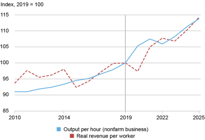
Official output per hour and public firms' real revenue per worker, both indexed to 2019 = 100. Both speed up after 2019.1 / 2
U.S. 1, or output per hour worked, is growing about twice as fast as it did in the 2010s. In a post on the New York Fed's Liberty Street Economics blog, economist Jeremy Pearce confirms this with company-level data. He then asks where the gains went. A good share went to corporate profit margins.
The turn
From 2010 to 2019, output per hour in the nonfarm business sector grew about 1.0 percent a year, according to the Bureau of Labor Statistics. In the late 1990s it had grown about 3 percent. From 2019 to 2025, growth rose to 2.2 percent.
Pearce checked this against 2, a database built from the annual 3 reports public companies file. He measured 4: sales adjusted for industry price changes, divided by employees. He left out sectors where productivity is hard to measure, such as finance, real estate, utilities and agriculture. Growth on this measure went from 0.7 percent a year to 2.2 percent, closely matching the official figures.
Where the money went
Higher revenue per worker could go to workers as higher pay, if firms compete for staff, or stay with firms as profit. Pearce tracks profit margins, the share of each sales dollar a firm keeps after costs. In the 2010s margins barely moved. Since 2019:
5, which subtracts only direct production costs, rose from about 34 percent of sales to 37 percent (1.3 percent a year).
6, which also subtracts overhead such as sales, administration and R&D, rose from about 16 percent to 18 percent (2.4 percent a year).
To put that in scale (illustrative numbers): a company with $10 billion in sales would keep about $200 million more in operating profit each year without selling anything extra. Pearce notes this fits with the long decline in the 7, the part of national income paid to workers.
R&D-heavy firms gained most
Firms that spent more on research and development relative to sales in 2019 saw larger margin gains afterward. A firm with 10 percent higher R&D intensity had about 0.7 percent faster operating-markup growth over 2019–2025. Firms that relied heavily on physical capital, like plants and machinery, showed no such pattern. Pearce reads this as evidence of returns to 8, meaning non-physical assets such as research, software and brands.
Caveats
The data covers only public companies, which tend to be large. The R&D link is a correlation, not proof of cause. The post also doesn't measure wages directly. Pearce leaves the main question open: are these wider margins a fair return on costly intangible investment, or "purely a windfall for firms"?
The news
U.S. 1 is growing at twice its 2010s pace. In a post on the New York Fed's Liberty Street Economics blog, research economist Jeremy Pearce uses company filings to show the speed-up in individual public companies as well as in national data. He then asks who is getting the extra output, and finds that a good share has gone to corporate profit margins.
A decade of disappointment, then a turn
After the Great Recession, productivity growth slowed. Nonfarm-business output per hour, the Bureau of Labor Statistics (BLS) headline measure, grew about 1.0 percent a year from 2010 to 2019. In the late 1990s it had grown about 3 percent. Manufacturing slowed the most. Over the same years, growth in revenue per worker at public companies also slowed.
From 2019 to 2025 the BLS measure grew 2.2 percent a year. That turn is the starting point for the post.
Checking the macro story with firm data
National statistics can't tell you which firms are driving a trend or where the money goes. Pearce uses 2, a database built from the annual 3 reports that public companies file with regulators. He covers firms in manufacturing and services from 2010 to 2025 and splits the data into two periods, 2010–2019 and 2019–2025. He leaves out agriculture, utilities, finance, real estate and public administration, because productivity in those sectors is known to be hard to measure.
His firm-level measure is 4: a firm's sales, adjusted for price changes using its industry's output prices, divided by its number of employees. Adjusting for prices matters because otherwise inflation alone would make revenue per worker look like it was rising. By this measure, growth went from 0.7 percent a year in 2010–2019 to 2.2 percent in 2019–2025. That closely matches the BLS figures. The first chart indexes both series to 2019 = 100, and both bend upward after 2019. Pearce's conclusion: "the labor productivity uptick is real."
Who gets the extra revenue?
More revenue per worker doesn't say who benefits. Pearce sets out two possibilities. If firms compete hard for workers, the gains show up as higher wages. If they don't, the gains stay with the firm as profit. Firm data can't track pay directly here, but it can track profit margins: profit divided by sales, or the share of each sales dollar a company keeps after costs.
There are two versions:
5 subtracts only the direct cost of making the product, called cost of goods sold.
6 also subtracts overhead: selling, general and administrative expenses. In Compustat this usually includes R&D.
In the 2010s, margins barely changed. Gross margins rose about 0.4 percent a year and operating margins were roughly flat. After 2019, both rose:
2019
2025
Annual growth
Gross margin
~34% of sales
~37%
1.3%
Operating margin
~16% of sales
~18%
2.4%
These are sales-weighted averages, so large firms count for more. To see the size of the change (an illustrative calculation, not from the post): a company with $10 billion in sales and a 16 percent operating margin earns $1.6 billion in operating profit. At 18 percent, the same sales give $1.8 billion. That is $200 million more per year without selling anything extra.
Pearce notes that wider margins fit with the long-running fall in the 7, the part of national income paid to workers. When a firm keeps more of each sales dollar, less of it goes to costs, and wages are part of those costs.
Which firms gained most?
Pearce then asks whether firms that invest in 8 gained the most. Intangibles are non-physical assets such as research, software, patents and brands. This follows earlier work by Pearce and a co-author, which found a puzzle: R&D intensity in manufacturing kept rising through the 2010s while productivity growth stalled.
The result: firms that spent more on R&D relative to sales in 2019 saw bigger margin gains afterward. A firm with 10 percent higher R&D intensity in 2019 had about 0.7 percent faster growth in operating markup over 2019–2025, and about 0.5 percent over 2022–2025. Capital intensity, meaning how much a firm relies on physical assets like plants and machinery, showed no similar significant pattern. Pearce reads this as a sign of returns to intangible investment rather than to physical capital. He links it to the strong results of high-tech and intangible-heavy firms since COVID.
Caveats
Public firms only. Compustat covers listed companies, which tend to be large. Private and small businesses are not included.
Correlation, not cause. The R&D finding is a prediction pattern. Firms with high R&D in 2019 may also have had market power, network effects or a good fit with pandemic-era demand. The post does not separate these explanations.
Measurement. Compustat employee counts usually cover a firm's whole global workforce, and revenue is a rough stand-in for output. The close match with BLS data is reassuring, but it does not prove the two measure the same thing.
No wage data. The post shows that margins grew. It does not show how much workers' pay grew over the same period, so the split between wages and profits is inferred, not measured directly.
Open question. Pearce says plainly that he can't yet tell whether the higher margins are a fair return on years of costly intangible investment or "purely a windfall for firms." He leaves that for future work.
Why it's worth watching
For anyone hoping that faster productivity will lift living standards, this is mixed news. The productivity gain looks real, which is good. But at least some of it is showing up in profits rather than pay. For investors, it suggests that recent earnings strength reflects real efficiency gains, concentrated in R&D-heavy companies. Whether those margins last depends on the question Pearce leaves open: whether they are a return on investment or a windfall.
Remember
Company-level revenue data and official statistics both show productivity growth jumping from about 1 percent a year to 2.2 percent after 2019.
Operating margins at public firms rose from about 16 percent to 18 percent of sales between 2019 and 2025.
High R&D spending in 2019 predicted later margin gains. Reliance on physical capital like plants and machinery did not.
Active listings by month compared with 2017–2019, showing the seasonal pattern and the shrinking gap to pre-pandemic levels.
Bill McBride of the 1 newsletter has posted part one of his mid-October 2026 housing overview. Its message: homes for sale are coming back, buyers aren't, and prices have stopped climbing.
Sales stuck near the bottom
For existing homes (resales, not new construction), McBride reports:
September sales were down 2.2% from a year earlier and "historically low."
The sales pace, measured as a 2 (seasonally adjusted annual rate, one month's sales adjusted for season and scaled to a year), has been very low for four years.
3 (homes for sale divided by the monthly sales pace) is at its highest in over a decade.
The median price is up 1.3% year over year, but McBride says it has already peaked for 2026.
Results vary widely by region. The public excerpt doesn't say where.
Listings: rising, but not from new sellers
Citing 4's September report, McBride gives these numbers:
1,162,000 active listings, up 1.9% from August and 5.4% from a year earlier, the fastest yearly growth in six months (August was 3.6%).
Inventory is now 9.1% below pre-pandemic levels (2017–2019), down from an 11.1% gap in August. That is the smallest gap since the pandemic.
5 were roughly flat from a year ago.
That last point explains the rise. Owners aren't listing more homes than last year, so the higher total comes from homes that stay on the market longer. Realtor.com's report title says price cuts hit a four-year high as mortgage rates topped 7%.
This also explains why supply can be at a decade high while inventory is still below 2019. Months of supply is a ratio, and sales have fallen further than listings. In an illustrative example, 10% fewer listings combined with 26% fewer sales still leaves more months of supply.
McBride notes that listings are seasonal. Expect them to stay flat for about a month and then drop near year-end. That drop is normal and not a reversal.
Builders absorb the hit
McBride calls 2026 "a difficult year for homebuilders." Many finished new homes are unsold, more homes than usual are under construction without buyers, and builders are cutting prices to clear stock. Builders carry loan and land costs on every unsold house, so they can't wait out a slow market the way homeowners can. Their discounts also compete with resales.
The open questions
Taken together, the market is loosening slowly, not crashing. The detailed supply figures and regional breakdown are behind a paywall. Part two, covering prices, rents and mortgage rates, should show whether the 1.3% price gain keeps shrinking.
Bill McBride of the 1 newsletter has posted the first half of his mid-October 2026 housing overview, covering inventory and sales. The second half will cover prices, rents and mortgage rates. The public part of the post gives a clear direction: homes for sale are slowly coming back, buyers are not, and prices have stalled. The more detailed supply and sales data sits behind a paywall, so this summary covers only what is public.
The headline numbers
McBride's summary for existing homes, meaning resales rather than new construction:
Sales in September were down 2.2% year over year and are, in his words, "historically low."
The sales pace has been very low for four years. He measures it as a 2 (seasonally adjusted annual rate). That takes one month's sales, adjusts for normal seasonal swings, and scales the result to a full year so different months can be compared.
3 is at its highest level in over a decade.
Inventory growth may have picked up again compared with a year ago.
The median sale price is up 1.3% year over year, but McBride says it has already peaked for 2026.
Conditions differ a lot by region. The public excerpt doesn't say which regions.
For context from earlier years: annual existing-home sales were about 4.1 million in both 2023 and 2024, compared with more than 5 million a year in 2017–2019. A four-year run near that level is what "historically low" refers to.
Listings: the clearest data in the public section
McBride cites 4's September 2026 monthly report, titled "Price Cuts Hit 4-Year Highs as Mortgage Rates Top 7%." Its figures:
5: 1,162,000
Up 1.9% from August
Up 5.4% from a year earlier, faster than August's 3.6% and the fastest yearly growth in six months
9.1% below typical pre-pandemic levels (2017–2019), down from an 11.1% gap in August. That is the smallest gap since the pandemic began.
The gap between the last two points matters. If sellers aren't listing more homes than last year, yet the total for sale keeps rising, the extra inventory comes from homes that stay on the market longer without selling. Inventory is growing because demand is weak, not because a wave of sellers has arrived. The report's title backs this up: price cuts at a four-year high are what sellers do when homes aren't moving. McBride doesn't spell out this reasoning in the public section. It follows from the numbers he quotes.
Why months of supply can be high while inventory is low
These two facts look contradictory: inventory is still below pre-pandemic levels, yet months of supply is at a decade high. Months of supply is a ratio, homes for sale divided by monthly sales, so it rises if the top grows or the bottom shrinks.
An illustrative example with round numbers (not McBride's data): in 2019, suppose 1.6 million homes were for sale and sales ran at 5.4 million a year, or 450,000 a month. That is about 3.6 months of supply. Now suppose inventory is 10% lower, at 1.44 million, but sales are down to 4 million a year, about 333,000 a month. Supply becomes about 4.3 months. Even with fewer homes for sale, the market has more slack, because sales fell faster than inventory.
That is today's market. Sales are the weak side, held down by mortgage rates above 7% and by owners who don't want to give up cheap pandemic-era loans.
Seasonality
McBride says the listings series is strongly seasonal. He expects active listings to stay roughly flat for about another month and then fall toward year-end, as they do every year. A drop in December wouldn't mean the trend has reversed. The useful comparison is year over year, and against the 2017–2019 baseline.
Homebuilders' difficult year
McBride calls 2026 "a difficult year for homebuilders." He lists three signs:
A large number of completed new homes still for sale, meaning finished houses with no buyer.
A larger than normal number of unsold homes under construction.
Builders cutting prices to clear inventory.
Builders work differently from individual sellers. An owner who doesn't get their price can take the house off the market and stay. A builder is carrying construction loans and land costs on every unsold unit, so it has to sell even if that means accepting less. That makes new-home prices and incentives an early sign of where the wider market is going. It also puts pressure on resale prices, because buyers can choose a discounted new house instead.
What it adds up to
Read together, the public data shows a market loosening slowly rather than collapsing. Inventory is rising and nearly back to pre-pandemic norms. Sales are stuck near multi-decade lows. Median prices are still slightly up from last year, but only by 1.3%, which is below typical inflation, so in real terms prices are falling slightly. Builders are absorbing most of the adjustment through price cuts.
What's missing
The detailed months-of-supply figures, the regional breakdown and the rest of the sales data are behind the paywall. The public section doesn't say which regions are weakest or give the exact months-of-supply number. Part 2, on prices, rents and rates, will show whether the 1.3% price gain keeps shrinking.
Remember
Inventory is rising because homes sit unsold longer, not because more owners are listing.
Months of supply is at a decade high because sales fell more than inventory did.
Builders with unsold finished homes are cutting prices, which puts pressure on resale values.
TiRADE chart: blue dots are threatened or announced tariffs, green dots are implemented ones, January 2025 onward.
The news
Economists at Brown University's 1 have recorded every time President Trump has put a specific number on a US 2 since January 21, 2025. The team is Şebnem Kalemli-Özcan, Can Soylu and Muhammed A. Yildirim. Their dataset, 3 ("Tariff Rates in Announcements, Declarations, and Events"), contains 749 statements covering 341 separate tariff changes.
Timothy Taylor, who writes the Conversable Economist blog, pointed readers to the project's main chart. He said it left him unsure "whether to laugh or cry."
What was counted
The researchers included every channel the president uses:
speeches, interviews and 4 (informal question sessions with reporters)
posts on 5, his social media platform
6, the documents that legally change rates
White House fact sheets
A single tariff often came up several times in different places, which is why there are about 2.2 statements for each actual change. Over roughly 21 months, that adds up to more than one numbered tariff statement a day.
What the chart shows
In the chart, blue dots are tariffs that were threatened or announced, and green dots are tariffs that were implemented. The two often don't line up. For a business that imports goods, a blue dot gives no guarantee about whether a rate will take effect, when, or at what level.
That matters because a tariff is a tax on imports. When the rate is unpredictable, companies face a cost beyond the tax itself. They may delay investments, rush shipments in before a deadline, or avoid long supplier contracts, even if the threatened rate never arrives. Taylor's post doesn't say what share of threats were carried out. Sources for each statement are on the TiRADE website.
Taylor's argument
Taylor separates the question of whether tariffs are wise from the question of how this policy has been run. He would "probably disagree" with raising tariffs broadly, and he says narrow, targeted tariffs need case-by-case judgment. His main point is that the chart shows no plan to judge at all. In his view, US tariff policy since early 2025 has been "a sputtering and erratic seat-of-the-pants shambles."
The dataset counts statements, not their economic effects. It doesn't measure how much trade each change covered, or whether the volatility showed up in prices or investment. Those are the next questions it could help answer.
The news
Three economists at Brown University's 1, Şebnem Kalemli-Özcan, Can Soylu and Muhammed A. Yildirim, have built a dataset of every occasion since January 21, 2025 on which President Trump "attached a number to a US 2, whatever the channel." They call it 3, short for "Tariff Rates in Announcements, Declarations, and Events." Timothy Taylor, who writes the Conversable Economist blog, highlighted the project's main chart and said it made him unsure "whether to laugh or cry."
What was counted
The researchers drew on every channel the president uses:
speeches, interviews and 4 (informal question sessions with reporters)
posts on 5, the president's own social media platform
6, the legal documents that actually change tariff rates
White House fact sheets and statements
Many rates were announced more than once in different places. A rate might be floated in an interview, repeated in a post, and later formalized in an order. So the researchers separate the raw number of statements, 749, from the number of distinct tariff changes those statements describe, 341. That works out to about 2.2 public statements per change. Over roughly 21 months, it also means a new numbered tariff statement more than once a day on average.
What the chart shows
The TiRADE figure plots each statement over time. Blue dots are tariffs that were threatened or announced, and green dots are tariffs that were implemented. The gap between the two colors is the point. When a rate is announced, an importer can't tell whether it will take effect, at that level, on that date, or at all. Taylor's post doesn't give a breakdown of how many threats became real tariffs, or how long the gap between threat and implementation usually was. The full details and sources for each statement are on the TiRADE website.
Why instability is a cost in itself
The article mostly leaves this step to the reader. Normally a tariff's economic effect is analyzed through its rate: who pays the tax, how much prices go up, how trade shifts to other countries. A volatile tariff regime adds a second cost on top of whatever rate is in force. Here is an illustrative example, not from the article: a retailer deciding whether to sign a year-long contract with a factory abroad has to price in a range of possible tariffs (say 10%, 25% or 50%) instead of one known rate. The usual responses are to wait, to stock up on inventory before a rate takes effect, or to pay more for flexible arrangements. All of them cost money, even if the highest rate never arrives. Economists studying trade policy uncertainty have linked these effects to lower investment.
Taylor's argument
Taylor keeps his view of tariffs separate from his view of how this policy has been run. He says he would "probably disagree with an overall plan to raise tariffs in broad ways." He would judge narrow, targeted tariffs "on a case-by-case basis." His criticism here is that there is no plan to evaluate at all. In his words, the chart shows US tariff policy since early 2025 has been "a sputtering and erratic seat-of-the-pants shambles" rather than a coherent strategy.
This is an argument about process, and it doesn't depend on whether tariffs are good or bad. Someone who favors higher tariffs could still agree that rates which are announced, changed and withdrawn this often make the policy harder to follow and less likely to achieve its own goals, such as persuading companies to move production back to the US.
What remains open
The post is short and leaves several questions open:
Follow-through rate. What share of announced tariffs were implemented, and at the announced level?
Measured effects. Did the volatility show up in import timing, inventories, prices or business investment? TiRADE records statements, not outcomes.
Weighting. A tariff on all imports from one major trading partner and a tariff on one narrow product each count as one change. The count of 341 doesn't show how much trade each change affected.
The dataset makes those questions easier to study, because it gives researchers a dated record of what was said and what was done.
Remember
About 2.2 public statements per real tariff change: the same rate is often announced several times before it takes effect.
A gap between threatened and implemented rates costs businesses money even if the threats never take effect.
Taylor criticizes how the policy was run, not tariffs as such: no coherent plan is visible to evaluate.
Tech workers' wages relative to similarly skilled peers elsewhere: a premium in the late 1990s, then a lasting gap below them.
Joining a hot industry at its peak can cost you over a whole career. That is the finding of a new study by Johan Hombert of HEC Paris, a French business school, and Adrien Matray of the Federal Reserve Bank of Atlanta. Joachim Klement summarises it and uses it as a warning for people switching into AI jobs today.
The boom
In the late-1990s 1, up to a quarter of all highly skilled US workers moved into tech and telecom. Internet businesses and new networks built on fibre-optic cable promised big rewards to founders, and ordinary employees were paid more than in similar jobs elsewhere. Much of the money behind the boom was cheap: debt, plus 2 and 3 (investment funds that buy stakes in private companies). When the bubble burst, that money stopped coming, many firms failed, and many people lost their jobs.
The numbers
The researchers compared tech workers' wages with those of similarly skilled workers in other sectors.
Late 1990s: people already in tech and people who joined during the boom earned 5–10% more than their peers.
By 2005: the premium had gone, and tech workers earned less than their peers.
About 15 years after the peak: people who joined tech before or during the bubble earned on average 7–8% less than comparable workers outside it.
Why: skills that expire
The losses weren't only among people who were laid off. Klement points out that even those who kept their jobs in the industry fell behind. Tech skills date fast. "Web designer" was a prized job around 2000 and barely exists now. Once the technology moved on, someone skilled at hand-coding web pages became less productive, and so less valuable to employers. Workers in other sectors kept more of their skills' value.
Klement's warning on AI
Klement argues the AI boom is a bigger bubble than the dot-com one, in both the stock market and the job market. If so, people taking higher-paid AI jobs now may be trading a short-term premium for lower pay over their careers.
What the summary leaves out
The post is short. It doesn't explain how "similarly skilled" peers were matched, whether pay figures include stock options, or how the lifetime cost adds up across the years of premium and penalty. It also doesn't show why AI skills would date the same way web design did. The parallel is Klement's argument, not a result of the study.
A new study by Johan Hombert of HEC Paris, a French business school, and Adrien Matray of the Federal Reserve Bank of Atlanta followed the pay of highly skilled Americans in the IT sector through the dot-com boom and bust. They found that the people who went into tech when it was hottest ended up worse off than similar people who stayed out. Joachim Klement wrote up the result in his newsletter as the third in a run of posts on AI and productivity. His message to anyone who has just switched into an AI job for the money is blunt: you may have cut your lifetime earnings.
The setup: a sector everyone rushed into
In the late 1990s, up to a quarter of all highly skilled US workers joined the tech and telecom sector. The draw was real. The internet and new communications technology, such as fibre-optic networks, offered entrepreneurs big potential rewards, and ordinary employees earned more than in comparable jobs in other sectors.
Klement stresses that much of the boom ran on cheap money: large amounts of debt, plus 1 and 2, funds that invest in private companies in return for ownership stakes. When the bubble burst in 2000–2002 and that money dried up, many companies went bankrupt and many more people lost their jobs.
The method in brief
The key comparison is between tech workers and similarly skilled workers in other sectors. This tries to hold the person constant, comparing for example two people with similar education and ability, and to measure only what the choice of sector did to their pay. The post doesn't say exactly how the researchers defined "similarly skilled" or what data they used. Readers who want those details will need the paper itself.
The results
The chart tracks the average wage of tech workers relative to their peers over time:
Late 1990s, at the peak: both long-time tech workers and boom-era newcomers earned 5% to 10% more than comparable workers in other sectors.
After the crash: the premium shrank quickly. By 2005, tech workers were earning less than their peers.
About 15 years after the peak: workers who joined before or during the bubble earned on average 7–8% less than similarly skilled workers elsewhere.
To see what that means over a career, here is an illustration (not from the study). Take two equally skilled workers whose peer benchmark pays $100,000 a year. Around 1999 the tech worker might earn $107,500, about $7,500 ahead. By the mid-2010s the same person might earn $92,500, about $7,500 behind. A few good years at the top don't make up for a decade or more of earning less. That is why Klement frames the finding in terms of lifetime earnings rather than any one year's pay.
The mechanism: 3
Layoffs are the obvious cost of a bust, but they aren't the main point here. Klement highlights that even workers who kept their jobs and stayed in tech fell behind. His explanation is that tech skills go out of date quickly. Around 2000, "web designer" was the skilled job of the moment. It hardly exists today. Someone very good at hand-writing the code behind web pages and designing them saw those skills lose value as the technology changed.
In economic terms, a worker's pay roughly tracks their productivity to an employer. When the tools change, the specific know-how built around the old tools becomes less useful, productivity in the new workplace falls, and pay follows. A worker in a slower-moving sector keeps more of what they know relevant for longer, so their pay keeps growing while the tech worker's falls back.
Klement's argument about AI
Klement goes further than the study. He argues that the current AI bubble is larger than the 4, both in the stock market and in the labour market. If he is right, the same pattern could repeat: high pay to draw people in now, then a correction, then a long period in which skills specific to today's AI tools lose value. He sums it up as "the grass isn't always greener on the other side."
Caveats and open questions
The source is a short newsletter post about a single chart, so a lot is left open:
Who left the sector? The post covers people who joined tech before or during the boom. It doesn't make clear whether those who later moved to other industries are counted in the 7–8% figure, or how they fared.
What counts as pay? In the dot-com era a lot of the "upside" came as stock options. The post refers to wages, and doesn't say whether equity gains or losses are included.
Lifetime total: the post gives yearly gaps, not a dollar estimate of lifetime losses. It also doesn't say whether the early premium is fully offset.
Does AI fit the pattern? The claim that AI skills will date as quickly as web design did, and that AI is a bigger bubble, is Klement's opinion and not a result of the study. Some AI-related skills, such as statistics, software engineering and data work, may hold their value better than skills tied to one tool.
Selection: people who rush into a booming sector may differ from those who don't in ways that are hard to measure. The post doesn't explain how the study deals with that.
For an individual, the practical lesson is narrower than "avoid AI jobs." A pay premium in a booming sector is partly payment for risk: the risk of a funding-driven bust, and the faster loss of value of skills tied to one technology. If you take such a job, it pays to keep building skills that will still be useful after the tools change.
Remember
Up to a quarter of highly skilled US workers moved into tech and telecom during the late-1990s boom.
Even tech workers who kept their jobs fell behind, because skills tied to specific tools lost value quickly.
That AI will repeat this pattern is Klement's argument; the study itself looks only at the dot-com era.
Epoch AI chart of AI company revenue, which surged after coding agents launched.1 / 4
In summer 2025, some analysts feared the AI data center boom could end like the railroad boom: in a crash, as in 1873. Noah Smith now revisits the idea. His verdict: there's no obvious bust in sight, but the stakes have risen because the builders are now borrowing.
What changed in a year
Back then, AI revenue was growing far more slowly than spending. The danger looked distant because the 1 were mostly paying cash. Those are the cloud giants like Amazon, Google, Meta and Oracle that build data centers.
Since then, spending has sped up, and revenue has sped up even more. Smith calls 2 AI's "killer app". These are tools like Anthropic's Claude Code and OpenAI's Codex, which write software with little supervision. They left Anthropic, and to a lesser degree OpenAI, "rolling in cash."
Bigger than the railroads?
Estimates of the boom's size are all over the place:
Economist Stijn Van Nieuwerburgh puts AI investment at 3.63% of 3, the size of the whole economy, against 2.24% for railroads. But the railroad boom lasted decades, and one dataset shows railroad spending peaking near 5.4%.
Banks and ratings agencies estimate lower AI figures. They count announced dollar spending, while Van Nieuwerburgh assumes the announced projects will cost more than companies expect.
Analyst Dylan Patel says AI tops 6% once you include chip factories, chips and energy.
Whichever number is right, Smith concludes that AI is now one of the two largest infrastructure booms in American history.
The real worry: debt
Hyperscalers used to fund data centers from the profits of their cloud and software businesses. The buildout has outgrown that. Bloomberg data shows they are now borrowing heavily. For every hyperscaler except Microsoft, 4 (cash left after investment) has gone negative or is expected to by late this year. Chipmakers like Nvidia and 5 are collecting much of the money.
Smith explains why debt changes the risk. If a company pays cash and AI revenue disappoints, its stock falls but its business carries on and eventually recovers. If it borrowed, it needs enough revenue to keep up its loan payments. Without that revenue, it could default, and defaults spread to lenders. That is how the railroad overbuild became the 6 and a decade-long depression.
The available text stops here. It doesn't include Smith's estimate of how likely a bust is, or totals for how much has been borrowed.
The worry, revisited
A little over a year ago, in summer 2025, some analysts feared the AI data center boom would end the way the railroad boom did in 1873: in a crash. Noah Smith covered the idea then. The concern was never that AI is useless. Even a technology that eventually produces huge growth can bankrupt the people who build its infrastructure, if they borrow more than they can repay before the payoff arrives.
At that point the danger looked distant. AI revenue was growing, but much more slowly than spending. Still, the 1 (the cloud giants that build data centers, like Amazon, Google, Meta and Oracle) were mostly paying with their own cash. The risk was about what might come later: if spending kept climbing and revenue didn't catch up, an 1873-style bust could follow.
Smith now checks back in. Two things happened, and they pull in opposite directions.
Revenue caught up, for now
First, revenue sped up even more than spending did. Smith calls 2 AI's "killer app". These are tools like Anthropic's Claude Code and OpenAI's Codex, which write and edit software with little hand-holding. With them, Anthropic, and to a lesser degree OpenAI, started "rolling in cash", according to Epoch AI data he cites.
So, as in summer 2025, Smith doesn't see an obvious bust coming soon. The difference is what's at stake. Companies are now borrowing far more, so any slowdown in AI's very fast revenue growth could set off a blowup.
How big is this boom? The numbers disagree
Smith calls the question of whether AI or the railroads is the bigger boom "pointless but fun", since the takeaway either way is that it's a lot of money. The estimates he collects vary widely:
Smith pins the AI gap mainly on cost assumptions. Banks and ratings agencies add up the dollar spending companies have announced. Van Nieuwerburgh starts from announced physical construction projects and estimates what they will cost. He comes out higher mainly because he assumes data centers will cost much more than the hyperscalers expect.
Smith's conclusion is that, whatever the right number, AI is now one of the two largest infrastructure booms in American history, "by a large margin." That is why people keep comparing it with the railroads, and why more skeptics are speaking up again. The railroad story ended with the 1873 crash and a depression that lasted roughly a decade.
The new part: debt
Smith's main point is that bubble talk is back, and the main reason is debt. In the early years, hyperscalers paid for data centers out of the large profits from their software and cloud businesses, and spent most of that cash on AI. The buildout has now outgrown what those profits can cover. Bloomberg data he cites shows them borrowing heavily to keep raising spending. For every hyperscaler except Microsoft, 4 (cash left after investment spending) has either already gone negative in recent months or is expected to by late this year.
The spending has been a windfall for chip companies such as Nvidia and 5 (Taiwan Semiconductor Manufacturing Company, the main contract chipmaker). Bloomberg figures show how much of the money ends up with them.
Why debt changes the risk
Smith spells out how the risk changes. Suppose a company pays cash for a data center and AI revenue disappoints. Its stock falls, but the core business keeps running, and profits eventually recover. The shareholders take the loss.
With borrowed money, the debt has to be repaid on schedule whether or not AI pays off. The more a hyperscaler borrows, the more revenue it needs just to stay solvent. If that revenue doesn't show up, it may default. Defaults spread to whoever lent the money, and that is how a railroad overbuild became a nationwide panic in 1873.
An illustrative example (not from the article): a company that pays $10 billion in cash for a data center that earns nothing loses $10 billion of value. A company that borrows the same $10 billion owes interest and principal on fixed dates. Without the revenue, that obligation can push it toward default.
What's left open
The available text ends here, partway through the argument. It doesn't give Smith's view on how likely a bust is, how much hyperscalers have borrowed in total, or who the lenders are. The size estimates also conflict and come from different methods, so read the GDP comparisons as rough. The firmest facts are about direction: spending is up, revenue is up faster for now, and the financing has moved from cash to debt.
Remember
Estimates of AI's size range from about 3.6% to over 6% of GDP, depending on cost assumptions.
Every hyperscaler except Microsoft has or soon will have negative free cash flow, so new spending is borrowed.
A boom paid for in cash hurts shareholders if it flops; a debt-funded one can cause defaults.
6, homes newly put on the market, were mostly unchanged from a year ago.
Stijn Van Nieuwerburgh (2026) puts AI investment at 3.63% of 3 (gross domestic product, the size of the whole economy) and railroads at 2.24%.
Those two figures cover very different time spans, because the railroad boom lasted decades. Data compiled by Justin Fox shows railroad spending peaking around 5.4% of GDP.
Data from the 1800s is patchy. Some sources give the railroad buildout much higher figures.
Banks and ratings agencies put AI spending well below Van Nieuwerburgh's figure.
Dylan Patel, a semiconductor industry analyst, says AI already tops 6% of GDP once you count all related infrastructure: chip-factory equipment, the chips themselves, and energy.