Wages Catch Up, Billionaires Move Out · Morning Gist
Tuesday, October 205 stories · 16 min
Wages Catch Up, Billionaires Move Out
Today's stories look at what really drives the numbers: incomes behind housing, enrollment behind Medicaid, and cheap power behind the data-centre buildout.
Picked from 53 new articles across 16 sources · arrow keys for other days
Today in 30 seconds
30s left
US home prices are still high relative to incomes. Wages are up 31% in five years, so expect flat prices like 1978–82, not a 2006-style crash. story 1 ↓
Tabarrok finds data centers aren't crowding out other investment. Real non-tech investment is still about 3% above 2023, and most of the rise in rates came before AI. story 2 ↓
Medicaid costs are climbing because enrollment went from 10% to nearly 30% of Americans. Elderly and disabled enrollees, 17%, account for half of spending. story 3 ↓
California's one-time billionaire tax may raise about $30 billion, not $100 billion, after departures. It could even lose money once other taxes leave too. story 4 ↓
A Swiss study finds new power near US data centres in 2022–25 came mostly from renewables and batteries, not gas. story 5 ↓
1/5Calculated Risk· CalculatedRisk by Bill McBride· Oct 19
US house prices remain high relative to incomes, despite falling from 2022 peak
Bill McBride compared a national house-price index with two income measures. Relative to incomes, prices are 7.5% to 11% below their 2022 peak but still well above the historical norm.
Why it matters · If incomes, rather than falling prices, close the affordability gap, buyers and owners should expect years of flat home values, not a crash or a rebound.
Know this first
Context from the editor, not the article · 29 sec
1 · Price-to-income ratios
Housing is affordable over the long run only if prices track what people earn. Divide home prices by incomes and you get a rough gauge: a ratio well above its historical median suggests prices have run ahead of buyers' means.
2 · Case-Shiller is an index
The S&P CoreLogic Case-Shiller National index follows repeat sales of the same homes. It reports price changes relative to a base year, not dollar prices. A ratio built from it shows relative changes, not dollars-per-dollar.
3 · The 1978–82 housing cycle
In the late 1970s and early 1980s, inflation and mortgage rates above 18% held nominal home prices roughly flat. Fast-rising wages cut inflation-adjusted prices without a crash. In 2006–2011, nominal prices fell about a quarter.
2/5Marginal Revolution· Alex Tabarrok· Oct 19
Tabarrok: data centers aren't crowding out other US investment
Economist Alex Tabarrok argues against Paul Krugman's claim that AI data-center spending is starving other investment. He says the charts behind it mislead, rate rises came mostly earlier, and tariffs better explain weak non-tech investment.
Why it matters · Whether the AI boom is propping the economy up or draining it shapes how you read GDP reports, interest rates and the risk if AI spending stops.
Know this first
Context from the editor, not the article · 27 sec
1 · What crowding out means
Crowding out is when one borrower's extra demand for funds pushes up interest rates enough that other projects become unprofitable and don't happen. It usually comes up in arguments about government deficits.
2 · The loanable funds model
A textbook model treats saving as the supply of loans and investment as the demand for them. The interest rate is the price that balances the two. More borrowing raises the rate, which cuts other borrowing and also draws out extra saving.
3 · Real rates and TIPS
A real interest rate is the rate after inflation. Yields on TIPS, US Treasury bonds whose principal rises with inflation, are the standard market measure of real rates.
3/5Conversable Economist· conversableeconomist· Oct 19
Medicaid costs are growing because more people are enrolled, not because each enrollee costs more
A Cleveland Fed study finds Medicaid's spending growth comes mainly from enrollment, which roughly tripled as a share of Americans since 1990. Inflation-adjusted spending per enrollee has barely changed.
Why it matters · Medicaid is close to a $1 trillion line in federal and state budgets, and how it gets cut depends on knowing what actually drives the cost.
Know this first
Context from the editor, not the article · 25 sec
1 · Medicaid versus Medicare
Medicare is federal health insurance mainly for people 65 and older. Medicaid covers low-income people. States run it under federal rules, and the federal government and the states share the cost.
2 · The 2014 expansion
The Affordable Care Act let states extend Medicaid to nearly all adults with incomes up to 138% of the federal poverty line. A 2012 Supreme Court ruling made this optional, so only some states did it.
3 · Managed care
Most Medicaid enrollees today are covered through private insurers. The state pays each insurer a fixed monthly amount per enrollee, and the insurer arranges and pays for that person's care.
4/5Marginal Revolution· Tyler Cowen· Oct 19
California's one-time billionaire tax may lose more revenue than it raises
Economists Benjamin Jaros and Joshua Rauh estimate that California's one-time 5% wealth tax on billionaires would raise about $30 billion. Income tax lost for good when billionaires leave would outweigh it, leaving the state about $38.9 billion worse off.
Why it matters · Wealth taxes keep coming back as a budget fix. Whether one actually brings in money depends on how many taxpayers leave and what other taxes leave with them.
Know this first
Context from the editor, not the article · 30 sec
1 · Wealth tax vs income tax
An income tax hits what you earn each year. A wealth tax hits what you own: stocks, private companies, property. Billionaires hold most of their fortune in assets, so their wealth is far larger than their yearly income.
2 · Residency decides who pays
US states tax the people who live in them. California has a top income tax rate above 13%. If a resident moves to a state with no income tax, such as Texas or Florida, California mostly stops collecting from them.
3 · Present value
Present value turns a stream of future money into one number today by discounting later years. A lower discount rate makes future losses weigh more. That is why the results depend on which rate you pick.
5/5Klement on Investing· Joachim Klement· Oct 19
US data centres sped up renewable and battery building more than gas
A Swiss study (Heiss et al., 2026) compared where US data centres went up with where power plants were built. Near data centres, renewable and battery building sped up much more than gas building did.
Why it matters · The AI power boom is often sold as a gas investment story. This study suggests that the cheapest new power, not politics, is deciding what actually gets built.
Know this first
Context from the editor, not the article · 29 sec
1 · Why data centres need power
AI and cloud data centres draw large amounts of electricity around the clock. A big new site can need as much power as a small city, so the local grid has to add generating capacity to serve it.
2 · The gas-boom assumption
The common view has been that this demand would be met by gas plants, because they produce steady power on demand. Wind and solar output rises and falls with the weather and time of day.
3 · Cost and batteries
New solar and wind farms are now often the cheapest power to build per unit of electricity. Large battery systems store their output for use when the sun or wind drops, which makes up for part of the variability problem.
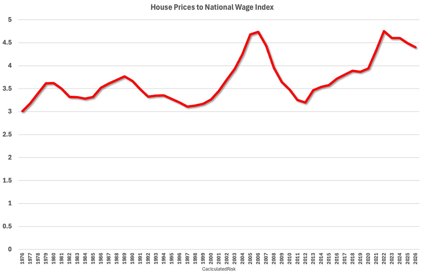
Case-Shiller national index divided by the average wage index since 1976: about 7.5% below the 2022 peak.1 / 2
Bill McBride of Calculated Risk updated his house-price-to-income ratios using fresh income data. By both measures he tracks, US home prices have come down from their 2022 peak relative to incomes, but they are still well above the long-run norm.
Why this is hard to measure
The idea is simple: compare home prices with what people earn. In practice, income data arrive with a long lag, and it's not obvious which income series to use. Average total income, for example, is pulled up by a few very high earners. The best-known price measure, the 1 (it tracks repeat sales of the same homes), is an index, not a price in dollars. So McBride divides the index by an income series. The result shows relative changes over time, not a literal "years of income per house."
Measure one: the wage index
The Social Security Administration's 2, an average of wages reported for US workers, came out last week for 2025:
$72,800.33, up 4.2% from $69,846.57 in 2024
The fifth straight year of strong gains
Wages up almost 31% over five years
McBride divides the mid-year Case-Shiller national index (data back to 1976) by the wage index divided by 1,000. He estimates 2026 wages by assuming a 4% rise. On this measure, prices are about 7.5% below the 2022 peak but still well above the median ratio.
Measure two: 3
The second ratio uses the Census Bureau's median household income through 2025, published in August 2026. He estimates 2026 with a 4.9% gain. Here prices sit about 11% below the 2022 peak, and again well above the historical median.
The argument: 1979, not 2006
McBride notes that five-year wage growth this strong last happened in the late 1970s and early 1980s. He sees that as another reason to compare today's housing market with the 1978–82 cycle, not with the 2000s bubble and bust. In that earlier period, high mortgage rates froze prices while fast-rising incomes slowly restored affordability.
His conclusion is that prices are too high for current incomes, and he expects them to "spend 7 years in 4." The phrase implies a long stretch of flat or slow-growing prices while incomes catch up, rather than a sharp fall.
Caveats
Both 2026 figures depend on assumed income growth. The wage index is an average, so high earners can skew it. Part of the post, including chart details, is behind a paywall. The seven-year timeline is McBride's judgment, and the free portion doesn't show how he arrived at it.
Bill McBride, who writes the Calculated Risk newsletter, has updated his house-price-to-income ratios with income data released over the last two months. He builds two versions from two different income series. Both say the same thing: relative to incomes, US home prices have fallen from their 2022 peak, but they remain well above the historical median. His forecast is that prices "spend 7 years in 1."
The problem: there's no clean ratio to read
A price-to-income ratio is one of the most basic checks on whether housing is overvalued. People buy homes out of income, so prices can't outrun earnings forever. Building the ratio is harder than it sounds, and McBride names the obstacles:
Lag. Most income data come out long after the year they cover. The 2025 numbers arrived in August and October 2026.
Which income? Average total income is skewed upward by a small number of very high earners. Medians avoid that problem but come from surveys with their own quirks.
Indexes, not prices. The most-watched national price measure, the S&P CoreLogic Case-Shiller National index, is a repeat-sales index. It tracks price changes on the same homes over time and is expressed relative to a base period, not in dollars.
The fix is to divide the price index by an income series. The resulting ratio has no natural unit, such as "five years of income." It is useful only compared with its own history: its median, its peaks and its troughs.
Ratio one: Case-Shiller over the 2
The National Average Wage Index (3) is published each October by the Social Security Administration. It averages the wages reported for US workers and is used to index Social Security benefits. The 2025 figures:
$72,800.33 in 2025, up 4.2% from $69,846.57 in 2024
The fifth consecutive year of strong wage gains
Up almost 31% over the past five years
McBride takes the mid-year value of the Case-Shiller national index (available since 1976) and divides it by NAWI divided by 1,000. Scaling the wage index down only keeps the ratio readable and doesn't change its shape. For 2026, the wage index doesn't exist yet, so he assumes a 4% increase.
Result: by this measure, house prices are about 7.5% below the 2022 peak but "still well above the median level."
Ratio two: Case-Shiller over 4
The second version uses the Census Bureau's nominal median household income, published through 2025 in August 2026. "5" means not adjusted for inflation, which fits a nominal price index. For 2026 he assumes a 4.9% gain.
Result: prices are about 11% below the 2022 peak and, again, well above the median historical ratio.
The two series differ in what they capture. NAWI is wages per worker. Household income includes every earner in a home and non-wage income such as benefits and investment income. Since 2022 they have also grown at different rates, so they give somewhat different distances from the peak. The free portion of the post doesn't break that difference down. The point is that two independent income measures agree on the direction and the rough size of the gap.
Why McBride points to 1978–82, not 2006
McBride notes that five-year wage growth near 31% matches the late 1970s and early 1980s. He calls this "another reason" to compare the current housing cycle with 1978–82 rather than with the 2000s bubble and bust.
The comparison matters because the two episodes resolved affordability in opposite ways:
2006–2011: Prices were inflated by loose lending, and the correction came through prices. The Case-Shiller national index fell roughly a quarter in nominal terms, with widespread foreclosures.
1978–82: Inflation was high and mortgage rates climbed above 18% in 1981. Sales slumped, but nominal prices mostly stalled instead of collapsing. Fast-rising incomes, plus inflation, did the work of bringing the ratio down.
Today's setup resembles the second case. Prices rose sharply in 2020–22, mortgage rates then jumped, and wages have been rising quickly. That combination favors a long stall over a crash.
What "purgatory" looks like in numbers
McBride's conclusion is that prices are "too high based on income levels," and that he expects them "to spend 7 years in purgatory." In practice that means a prolonged period of flat or slow nominal price growth while incomes rise underneath them.
An illustrative calculation, not from the article: suppose nominal prices stay flat and incomes grow 4% a year. Each year the ratio falls by about 4%. After seven years incomes are up about 32% (1.04⁷ ≈ 1.32), so the ratio is about 24% lower. Inflation-adjusted prices fall a lot, while the sticker price of a home barely moves. That is how affordability can improve without a crash.
Caveats
The 2026 points are estimates. The 4% wage and 4.9% median-income assumptions affect the latest reading. Slower income growth would make the ratio look worse.
Averages skew. NAWI is an average, so gains concentrated among high earners can flatter it relative to what typical buyers earn.
Ratios ignore financing. A price-to-income ratio leaves out mortgage rates, which drive the monthly payment buyers actually face. The same ratio is far less affordable at 7% than at 3%.
Paywall. Part of the post, including chart commentary, is for paid subscribers. The free section doesn't explain how McBride arrived at seven years specifically, so treat that figure as his judgment, not the output of a model.
The open question is whether incomes keep rising at the 4–5% pace these estimates assume. If they do, the gap closes slowly through income growth. If wage growth slows sharply, the stall either lasts longer or prices have to give.
Remember
Average US wages rose 4.2% in 2025 and almost 31% over five years, a pace last seen around 1980.
Price-to-income ratios are 7.5% to 11% below the 2022 peak, depending on which income measure is used.
Rising incomes can close an affordability gap without a price crash, as happened in 1978–82, not 2006–11.
The widely shared chart: data-center spending up $51 billion against a $120 billion fall elsewhere.1 / 4
Paul Krugman and others have been arguing that heavy spending on AI data centers is crowding out investment in the rest of the US economy, meaning it soaks up funding that other businesses would have used. Alex Tabarrok, an economist at George Mason University, says on 1 that the charts behind this claim don't show it.
The arithmetic problem
One widely shared chart, from commentator Steven Rattner, showed data-center construction spending up $51 billion while other investment fell $120 billion. Tabarrok notes that $51 billion of spending can't crowd out $120 billion. In the standard 2, where savers supply money and investors borrow it, crowding out is less than one-for-one. New borrowing raises interest rates. Higher rates discourage some other investment, but they also pull in more saving. So other investment falls by less than the new spending adds.
Shares versus dollars
Krugman used a broader chart: all "tech" investment against all other investment, each as a share of 3. That measure of tech investment rose about $539 billion over a similar period, roughly ten times the data-center figure. It counts far more than data centers.
Shares can also mislead when the economy is growing. If tech's share rises, other investment's share has to fall, even if other investment is growing in dollars. Tabarrok redrew the same data in inflation-adjusted dollars. From the second quarter of 2023 to the second quarter of 2026, real tech investment rose about 46% and other real investment rose about 3%. Other investment has slipped since its 2024 peak but is still above where it started.
Tabarrok grants that this doesn't rule out crowding out completely. Other investment might have grown faster without the AI boom. But these charts can't test that.
Interest rates don't fit the story
If AI borrowing were crowding out other investment, 4 (rates after inflation) should have jumped during the boom. Most of the rise came earlier. The 10-year 5 yield, the market's main gauge of real rates, went from −1.00% in late 2021 to 1.49% in late 2022. Over the periods in the Rattner and Krugman charts, it rose only 0.5 and 0.68 percentage points. Real rates of about 2–3% are close to historical norms. Rates also rose across other rich countries, even though most AI spending is in the US.
His alternative
Tabarrok's own explanation is that two things are happening at once. Tariffs, uncertainty and the fading of Biden-era subsidies have weakened investment outside tech, while AI spending has kept total investment up. In his view, AI investment is "a bright spot" in an otherwise weaker economy.
Paul Krugman and a number of other commentators have argued that the boom in AI data-center construction is crowding out investment everywhere else in the US economy. The idea is that money and resources poured into server farms are no longer available for factories, offices and equipment. Alex Tabarrok, a George Mason University economist who co-writes the blog 1, says the charts used to support this claim don't show it. He offers a different reading: AI spending is holding total investment up while other forces drag down everything else.
What crowding out is supposed to look like
The textbook mechanism is the 2. Think of saving as the supply of loans and investment as the demand for them, with the real interest rate (the rate after inflation) as the price that clears the market. Tabarrok's textbook, Modern Principles, written with Tyler Cowen, presents this with government borrowing as the new demand. He notes the diagram works the same way when tech companies are the new borrowers.
When a big new borrower arrives, the demand curve shifts out and the interest rate rises. That higher rate does two things:
Some other projects no longer pay off at the higher rate. That lost investment is the crowding out.
Households and firms save more, because saving now earns more, so the pool of funds gets bigger.
Because of the second effect, crowding out is "generically less than 1 to 1." Here is an illustration with made-up numbers: if tech firms borrow an extra $50 billion, the higher rate might draw out $20 billion of new saving. Other investment then falls by about $30 billion, not $50 billion.
Tabarrok adds that economists usually reserve "crowding out" for government borrowing. Private borrowers face a market test, so funds moving to them from lower-return uses is a gain, not a cost. He sets this point aside for the argument.
Problem one: the numbers don't add up
The chart that started the debate came from Steven Rattner, a financier and commentator. It showed data-center construction spending up $51 billion while other investment fell $120 billion. Under the model above, $51 billion of new spending can't crowd out more than $51 billion of other investment, let alone $120 billion. Something else has to be pushing other investment down.
Problem two: a different, much larger measure
Krugman didn't flag this issue. He used his own chart instead, comparing all "tech" investment with all other investment, each as a share of 3 (gross domestic product, the total value of what the economy produces). The ratios look more plausible, but the tech series rises about $539 billion over a similar two-plus-year period, roughly ten times Rattner's data-center figure. That's a much broader category than data centers or AI as usually defined. Tabarrok says that's a legitimate thing to study, but Krugman is borrowing the public's unease about data centers to make a claim about something larger.
Problem three: shares versus dollars
Shares of GDP can create a false picture. If tech investment's share goes up, other investment's share tends to go down. That can happen even when both are growing in dollars, as long as GDP itself is growing. Tabarrok redrew the same data in real (inflation-adjusted) dollars:
From Q2 2023 to Q2 2026, real tech investment rose about 46%.
Over the same period, real other investment rose about 3%.
Other investment has weakened since its 2024 peak but is still above its starting level.
He's careful about what this shows. It doesn't rule out crowding out, because other investment might have grown faster without the tech boom. But the argument has retreated a long way. It started as a claim of an absolute decline, then became a decline relative to GDP, and is now a claim about a 4 (what would have happened without the boom). These charts can't identify that counterfactual.
Problem four: interest rates moved at the wrong time
Crowding out works through higher interest rates, so rates should rise when the borrowing does. Tabarrok uses 5 yields, the return on Treasury bonds indexed to inflation, as the measure of real rates. The average 10-year TIPS yield went from −1.00% in late 2021 to 1.49% in late 2022, before the AI investment boom. Over the periods in the Rattner and Krugman charts, real rates rose only 0.5 and 0.68 percentage points. Tabarrok calls that "relatively small potatoes" for a crowding-out story.
Today's real rates of roughly 2–3% are in line with historical averages. In his words, "if there are good projects they can be funded."
He offers several possible reasons for the earlier rise:
recovery from unusually low pandemic-era rates
federal government borrowing
people saving less today because they expect AI to make them richer later
On the last point, he jokes about AI workers who have reportedly taken up smoking because they expect a future cure for lung cancer.
Real rates have also risen across advanced economies, even though most AI spending is in the US. Capital markets are global, and the world's pool of savings is much larger than America's. That makes it harder for US data-center borrowing alone to squeeze US investment.
His alternative explanation
Tabarrok thinks two separate things are happening at once. Investment outside AI and tech has been weakened by tariffs, policy uncertainty, and the fading of subsidies from two Biden-era laws: the 6, which funds semiconductor manufacturing, and the 7, which funds clean energy. AI investment, by contrast, has supported total investment. In his reading, AI spending is "a bright spot in what would otherwise be a more negative economy."
What remains open
The post is short and leaves gaps. It doesn't publish data sources or definitions for its redrawn chart. It doesn't measure how much tariffs or expiring subsidies have actually cut investment. And it can't settle the counterfactual it raises itself. Crowding out can also happen through real resources rather than money: electricians, power-grid capacity, transformers and construction crews all have limited supply. A rate-based argument doesn't address those limits, and the post doesn't discuss them. Tabarrok's case is mainly that the evidence offered so far is weak. He doesn't claim to prove that no crowding out is happening.
Remember
Textbook crowding out is less than one-for-one, because higher rates also draw out more saving.
Charts of GDP shares can show one category shrinking while it is still growing in real dollars.
Most of the rise in real rates happened in 2021–22, before the AI investment boom began.
Medicaid enrollment as a share of Americans has risen while real spending per enrollee stayed roughly flat.1 / 2
Medicaid spends close to $1 trillion a year, almost one in five dollars of all US health spending. About 65% comes from the federal government and the rest from the states. A new analysis by James Hamlette and Karen Kopecky of the Federal Reserve Bank of Cleveland, summarized by economist Timothy Taylor, explains why the bill keeps rising: more people are covered.
Enrollment, not cost per person
In 1990 about 10% of Americans were on Medicaid. Today it's approaching 30%. Average spending per enrollee, adjusted for inflation, has barely changed since 1990. Medicaid's growth is not mainly a story of rising medical prices. It's a story of a program that covers far more people.
Who joined, and when
The groups driving enrollment growth changed over time:
Before 2000: children and their families.
2000–2013: adults, both childless non-disabled adults and disabled adults. Working and non-working adults rose by similar amounts.
Since 2014: the 1 expansion. Participating states opened Medicaid to adults earning up to 138% of the 2, very roughly $21,600 a year for a single person in 2025. Most of this growth has been working adults.
Spending is concentrated
Elderly and disabled enrollees are 17.3% of Medicaid's members but just over half its spending, mostly for nursing homes, long-term care and chronic illness. By our rough calculation from those figures, each of them costs about five times as much as the average for everyone else.
Why 3 may save little
The main proposals to hold down Medicaid costs would require recipients to work. Congress put work requirements for expansion adults into law in 2025. Taylor argues the savings will be small. Non-disabled, non-elderly adults account for only about 15.8% of Medicaid spending, and many of them already work.
As an illustration (our numbers): a 10% cut in spending on that group would save about 1.6% of Medicaid's total. The expensive groups would be untouched.
Where to look instead
Taylor suggests studying how states design Medicaid 4. In that system, states pay private insurers a fixed monthly amount per enrollee to cover each person's care. He cites a Spring 2026 Journal of Economic Perspectives paper by Mark Shepard and Jacob Wallace on the "5." In that model, states choose which insurers may take part, then let them compete for enrollees. (Taylor is the journal's managing editor.) The authors say state designs vary widely and the evidence on what works is thin. So this is a direction for research, not a savings estimate.
Medicaid spends close to $1 trillion a year. About 65% comes from the federal government and the rest from the states. That is almost one in five dollars of all US health spending, a bit less than Medicare at about $1.2 trillion. Timothy Taylor's Conversable Economist blog summarizes a new analysis by James Hamlette and Karen Kopecky of the Federal Reserve Bank of Cleveland, "Who's Driving Medicaid's Enrollment Growth?" (October 13, 2026). Their answer to why the bill keeps rising is simple. Many more people are covered.
What Medicaid pays for
Medicaid is joint federal-state health insurance for eligible low-income people. Groups that can qualify include children, pregnant women, low-income elderly and disabled people, and adults in low-wage jobs. Federal rules require states to cover certain services:
inpatient and outpatient hospital care
physician services
nursing home care
mental health services
preventive care for children
States may also choose to cover prescription drugs, dental care, and home- and community-based care. Because each state makes different choices on top of the federal minimum, "Medicaid" is really about 50 different programs.
Enrollment, not cost per person
Medicaid outlays per US resident were four times their 1990 level in 2024, citing the Congressional Research Service. (The post does not say whether that figure is adjusted for inflation.) The authors break that growth into two parts:
Coverage: In 1990 about 10% of Americans were on Medicaid. The share is now approaching 30%.
Cost per enrollee: Average spending per enrollee, adjusted for overall inflation, has barely moved since 1990.
This matters because health spending is usually described as a price problem: medical inflation, expensive new treatments. For Medicaid as a whole, the cost of covering each person has roughly kept pace with prices in general. The growth comes from how many people the program covers.
Who drove the growth, decade by decade
Hamlette and Kopecky find that the groups behind enrollment growth changed over time:
Before 2000: mainly children and their families.
2000 to 2013: mainly adults, both childless non-disabled adults and disabled adults. The increase was roughly even between working and non-working adults.
Since 2014: the 1 expansion. States that opted in extended coverage to adults earning up to 138% of the 2. For a single adult in 2025 that was very roughly $21,600 a year. Growth in this period has come mainly from working adults.
Enrollees and costs don't match up
Average cost per enrollee hides big differences between groups. Elderly and disabled people make up 17.3% of Medicaid enrollees but just over half of spending. They need nursing homes, long-term care and treatment for chronic conditions.
A rough calculation (ours, using the post's figures) shows the gap:
Elderly and disabled: about 51% of spending divided by 17.3% of enrollees gives a ratio near 3.
Everyone else: about 49% of spending divided by 82.7% of enrollees gives a ratio near 0.6.
So an elderly or disabled enrollee costs roughly five times as much as the average for everyone else.
Why 3 may save little
Taylor applies this to current policy. The main proposals to hold down Medicaid costs would require recipients to work. Congress wrote work requirements for expansion adults into a 2025 budget law, set to take effect around the end of 2026.
Taylor argues the savings are likely to be limited, for two reasons:
Non-disabled, non-elderly adults, the group these rules target, account for only about 15.8% of Medicaid spending.
Many of them already work. Since 2014, working adults have driven most enrollment growth.
An illustration (our numbers, not the article's): suppose work requirements cut spending on this group by 10%. That would save about 1.6% of total Medicaid spending, around $16 billion on a roughly $1 trillion program. The big cost centers, elderly and disabled enrollees, would be untouched.
Where Taylor would look instead
Taylor suggests a more useful approach: study how states design their programs, especially 4. Under managed care, the state pays private insurers a fixed monthly amount per enrollee, and the insurer handles and pays for that person's care.
He points to Mark Shepard and Jacob Wallace's article "Understanding Medicaid Managed Care: The Procured Competition Model," in the Spring 2026 Journal of Economic Perspectives. Taylor is the journal's managing editor, which readers should keep in mind. In the model they describe:
The state runs a procurement to choose which insurers may take part.
Those insurers then compete to enroll beneficiaries.
The state controls who gets in, how the insurers compete, and how enrollees choose among them.
Shepard and Wallace say states set up these programs in very different ways, and there is little evidence on which designs work. They call this a promising area for research.
What's left open
The post is short and leaves several gaps:
It does not say what the remaining third or so of spending goes to. Children are the likely answer, but that is an inference.
It does not reconcile the fourfold rise in per-resident spending with the flat cost per enrollee. Partly this is a matter of nominal versus inflation-adjusted dollars, which the post doesn't spell out.
It offers no estimate of what better managed-care design might save. The research it cites says the evidence doesn't exist yet.
The firm conclusion is narrower: Medicaid's cost is mostly about how many people it covers. Within that, a small group of elderly and disabled enrollees accounts for most of the spending.
Remember
Inflation-adjusted Medicaid spending per enrollee has been roughly flat since 1990. Rising enrollment explains most of the growth.
Elderly and disabled enrollees, 17.3% of members, account for just over half of Medicaid spending.
Work requirements target adults who account for only about 15.8% of spending, and many of them already work.
Economists Benjamin Jaros and Joshua Rauh have a new 1 (National Bureau of Economic Research) working paper on the 2026 California Billionaire Tax Act. The act is a one-time 5% tax on the worldwide 2 of people worth more than $1 billion. The authors argue that it will probably cost the state money overall.
Tyler Cowen highlighted the paper on Marginal Revolution and called the issue "a good litmus test for who still thinks like an economist."
Why the base is shrinking
The headline estimate is that the tax collects about $30 billion, within a range of $28–36 billion. An earlier projection by Galle and coauthors (2025) put the figure at $100 billion, so the new estimate is less than a third of that. The authors give three reasons for the gap:
Billionaires are already leaving. Using the Forbes Billionaire List, news reports on where billionaires own homes, and public announcements of moves, the authors find that confirmed departures have already removed nearly 30% of the taxable wealth.
Legal risk. They apply a "3," which shrinks expected revenue by the chance the tax is struck down or stuck in court.
Outside evidence. Their range matches existing research on how much reported wealth shrinks when wealth taxes rise.
The bigger loss: income tax
The key point is timing. The wealth tax is paid once. Income tax from a resident billionaire comes in every year. The authors estimate that California's billionaires pay $3.3–5.8 billion a year in state income tax. When one moves to a state with no income tax, that money is gone for good.
Here is an illustrative example, not the paper's numbers. Losing $1.5 billion a year in perpetuity, discounted at 4%, is worth about $37.5 billion today. That is more than the entire one-time wealth tax haul.
The authors' central result is a 4 of negative $38.9 billion. Net 5 is all future gains and losses added up and converted into today's dollars.
How sure are they?
The outcome depends on uncertain revenue and on which discount rate you choose. So the authors ran 100,000 simulations across plausible combinations of both. 85% of them came out negative for the state. That leaves roughly one in seven where the tax doesn't lose money.
Caveats
This is a working paper, not yet peer reviewed. The post gives only the abstract, so it doesn't break the gap from $100 billion down by cause. It also doesn't say whether the result includes departures still expected or only those already confirmed. Much depends on whether departures really are permanent.
The news
A new 1 (National Bureau of Economic Research) working paper by Benjamin Jaros and Joshua Rauh models the revenue from the 2026 California Billionaire Tax Act. The act is a one-time 5% tax on the worldwide 2 of individuals worth more than $1 billion. The authors conclude it will probably leave California worse off. Their central estimate is that it collects about $30 billion, within a range of $28–36 billion. An earlier projection by Galle and coauthors (2025) put the figure at $100 billion, so the new estimate is less than a third of it. Counting the state income tax lost when billionaires move away, the authors estimate the act's 3 to state revenues at negative $38.9 billion.
Tyler Cowen, who flagged the paper on Marginal Revolution, calls the issue "a good litmus test for who still thinks like an economist." The post itself is just the paper's abstract plus that line. The detail below comes from the abstract alone.
Why scoring a wealth tax is hard
A simple revenue estimate multiplies the tax rate by the base. Here the base is the total net worth of California's billionaires. At 5%, a $100 billion yield implies about $2 trillion of taxable wealth. That arithmetic assumes the base stays put, and three things can shrink it:
Migration. Wealthy people can change their residence before the tax applies. A billionaire who leaves takes their whole fortune out of the base.
Litigation. Wealth taxes on worldwide assets invite legal challenges. If part of the tax is struck down or tied up in court, some of the expected money never comes in.
Spillovers to other taxes. A departed billionaire stops paying California income tax every year after leaving, not just once.
The third point drives the paper's main result. The wealth tax is collected once. A lost income tax payer is lost every year.
How the authors estimated it
Jaros and Rauh used three main sources:
The Forbes Billionaire List, to measure the size of the base.
News reports on billionaires' California homes, to judge who is really a resident.
Public announcements of billionaires leaving the state.
From these they say confirmed departures have already removed nearly 30% of the wealth tax base. They then apply a "4" to what remains, which shrinks the expected revenue by the chance that the tax doesn't hold up in court. They check the result against existing research on the 5 of the wealth tax base, meaning how much reported wealth shrinks as wealth tax rates rise. They say several methods land in the same $28–36 billion range. The abstract does not say how big the litigation discount is. It also doesn't say how much of the gap from $100 billion comes from migration, the legal discount, or differences in how the base is measured.
The income tax side
The authors estimate that California's billionaires pay $3.3–5.8 billion a year in state income taxes. Those payments recur, so losing them permanently has a large 6.
An illustrative example (these are not the paper's numbers). Suppose departing billionaires had paid $1.5 billion a year in income tax. Treated as a permanent loss and discounted at 4%, that stream is worth about $1.5B ÷ 0.04 = $37.5 billion today. That alone is more than the wealth tax's one-time $30 billion. A lower discount rate or larger departures widen the gap. This is the logic behind the paper's conclusion that lost income tax "more than offsets" the one-time collection.
How confident is the result?
The answer turns on two uncertain inputs: how much the wealth tax actually raises, and what discount rate to use. So the authors ran 100,000 simulations across plausible combinations of the two. In 85% of them, the net present value to the state is negative. By the authors' own reckoning, the tax still breaks even or better in about one case in seven.
What the abstract leaves open
What the $38.9 billion counts. The abstract does not say whether that figure includes only billionaires who have already left, or also departures the authors expect later.
Permanence. The result treats lost income tax as permanent. Some people come back, and fortunes change over time, so the length of the loss matters a lot.
Who disagrees. The $100 billion estimate from Galle et al. is the main counterpoint. The post doesn't present their side or any response to this paper.
Status. This is a working paper, so it has not been peer reviewed. Its departure data comes from public announcements, which may miss quiet moves or count moves that are partly for show.
The general lesson goes beyond California. A tax that people can avoid by moving should be judged on all the revenue that leaves with them, not on the size of the base before anyone reacts.
Remember
A one-time tax collected once can be outweighed by income tax lost every year after the taxpayers leave.
Confirmed departures alone have removed nearly 30% of the taxable wealth before any money is collected.
The result depends on the discount rate, but 85% of 100,000 simulated scenarios still show a net loss.
US data centre capacity at end-2025, concentrated in Texas, Virginia, Ohio and Nevada.1 / 3
The news
The usual story is that the American AI boom runs on gas: data centres need steady power around the clock, and gas plants provide it. Joachim Klement highlights a Swiss study, 1, which finds that this is mostly not what happened between 2022 and the end of 2025.
What the study did
The researchers first mapped where US data centres were built. Building was concentrated in states with the cheapest energy: Texas, Virginia, Ohio and Nevada. Next they tracked new power plants nationwide. Most new generating 2 came from renewables, and gas made up only a small share.
Then they put the two together and compared areas that got a data centre with areas that didn't:
Renewables and batteries: In data centre areas, building of renewables and battery electric storage systems (3, grid-scale batteries) sped up much more than elsewhere.
Gas: Gas building also sped up near data centres, but by much less than in areas without them.
Klement's reading is that a new data centre raises local power demand, and that new supply is "more likely than not" to come from renewables and batteries. His explanation is cost: new renewable capacity is cheaper to build than new gas plants, so it gets built despite federal policy that favours fossil fuels. "Money talks," he writes. Texas leads the country in wind and solar, yet you'd never guess it from the local politics.
Europe shows the same pattern. Its biggest data centre hubs, the UK and Spain, have paired data centre growth with spending on renewables and batteries.
Caveats
The post is three charts and a few paragraphs, and it gives no figures. It only describes which way the charts point. The following doubts are the editor's, not Klement's:
Capacity isn't output. The charts appear to count maximum rated output. Solar delivers only about a quarter of that over a year, while gas can run much more of the time. Most new capacity being renewable doesn't mean most new electricity is.
Which way the link runs. Data centres chose places with cheap power, which in Texas and Nevada often means wind and solar. Cheap renewables may be attracting data centres as much as data centres are attracting renewables.
Timing. Gas turbines have long order backlogs. Gas plants planned for the AI boom may not appear in data that ends in 2025.
For investors, this is a credible challenge to the idea that "AI means gas". It is not yet proof against it.
The claim
The usual story about AI's power demand in the US is that data centres are reviving gas power. Joachim Klement points to a study from Switzerland, 1, which suggests the opposite. Between 2022 and the end of 2025, places that got a new data centre saw renewables and battery storage build out much faster than gas.
Europe is less of a surprise. Klement notes that its biggest data centre hubs, the UK and Spain, have paired data centre growth with more spending on renewables and batteries. The US was the place where gas was expected to win.
Why gas was the expected winner
A data centre runs around the clock, and it wants power that is always there. Gas plants can be switched up or down on demand. Solar and wind can't, since their output depends on the weather and the time of day. Policy also seemed to favour gas. Klement mentions the "best efforts of the current US government". That is a reference to the administration's support for fossil fuels and its rollback of support for clean energy, which included cuts to wind and solar tax credits in 2025.
What the study did
The authors did three things.
They mapped where data centres went. Building from 2022 to 2025 was concentrated in states with the cheapest energy: Texas, Virginia, Ohio and Nevada.
They tracked national power plant additions. Most new US generating 2 came from renewables. Gas made up only a small fraction. Their chart marks the launch of 3 in late 2022 as a reference point for the AI boom.
They put the two together. They compared power building in areas that got a data centre with areas that didn't, before and after the boom.
What they found
Renewables and batteries: In data centre areas, building of renewables and battery electric storage systems (4, grid-scale batteries) sped up much more than in areas without one.
Gas: Gas building also sped up in data centre areas, but by much less than it did in areas without data centres.
Klement concludes that a data centre arriving in your area raises local power demand, and that this demand "is more likely than not" to be met by renewables and batteries rather than gas. His explanation is simple: "money talks." New renewable capacity is cheaper to build than new gas plants, so developers build it whatever the political mood.
He ends with a jab: "talk to anyone in Texas, and you wouldn't know any of it." Texas is the US leader in both wind and solar, yet it is politically identified with oil and gas.
What the article doesn't tell you
The post is short. It gives no actual figures: no megawatts, no growth rates, no gap between data centre and non-data-centre areas. It only describes the direction shown in the charts. Several questions are worth keeping in mind. These are the editor's caveats, not Klement's:
Capacity is not energy. The charts appear to count capacity, meaning a plant's maximum rated output. A solar farm typically runs at about a quarter of its rated output over a year. A gas plant can run far more of the time. So 1 gigawatt of new solar delivers much less electricity than 1 gigawatt of gas. "Most new capacity is renewable" does not mean "most new electricity is renewable."
Correlation and site selection. Data centres went to places with cheap power. In Texas and Nevada, that cheap power is largely wind and solar. Some of the link may run from cheap renewables to data centres, not the other way round. The article doesn't say how the study handles this.
Timing. New gas turbines face long manufacturing waits, so gas plants planned for data centres in 2024–25 may not show up in completed capacity until later. A study ending in 2025 could understate gas.
What "area" means. The article doesn't say how regions are defined. That choice affects how cleanly the two groups can be compared.
Why it matters for investors
If the finding holds up, the economics are pulling the AI power buildout towards solar, wind and batteries, despite the politics. That matters for anyone weighing utilities, power developers or energy-transition funds against a plain "AI means gas" story. Still, the evidence here is three charts and a one-paragraph summary of a study. It is better read as a challenge to the conventional wisdom than as proof that the conventional wisdom is wrong.
Remember
Near new US data centres, gas building rose by less than it did in areas without data centres.
The study counts plant capacity. Solar's lower output per rated megawatt means its share of actual electricity is smaller.
Cost of new building, not federal policy, appears to be deciding what kind of power gets added.