Houses, pensions and billionaires who fell for it · Morning Gist
Wednesday, October 285 stories · 15 min
Houses, pensions and billionaires who fell for it
Social Security's real shortfall, home prices that keep losing to inflation, German exporters losing ground to China, and why smart money still gets fooled.
Picked from 57 new articles across 16 sources · arrow keys for other days
Today in 30 seconds
30s left
Social Security's trust fund is projected to run out in 2032, but payroll taxes would still pay about 78% of benefits. Planning around 70% is sensible. story 1 ↓
US home prices rose 2.1% over the year but have fallen after inflation for 15 straight months. Chicago is up 6.7%, Seattle down 2.0%. story 2 ↓
New home sales fell to a 676,000 annual pace in September, beating forecasts. Builders hold 8.4 months of supply, and unstarted homes are at a record. story 3 ↓
From 2012 to 2024, Germany lost export share to China faster than the rest of Europe, mostly in cars, machinery and electrical and medical equipment. story 4 ↓
Theranos fooled billionaires because intelligence doesn't help people spot their own biases, Ben Carlson argues. Check investments yourself instead of trusting big names. story 5 ↓
1/5Of Dollars and Data· Nick Maggiulli· Oct 27
Social Security won't vanish; planning on 70% of benefits is reasonable
Nick Maggiulli works through Social Security's finances and its benefit formula. He concludes that younger workers should plan on getting about 70% of their estimated benefit, not zero, and shows how to build that into a retirement plan.
Why it matters · How much Social Security you expect changes how much you need to save, often by hundreds of thousands of dollars. Assuming zero or assuming 100% are both costly mistakes.
Know this first
Context from the editor, not the article · 28 sec
1 · How Social Security is funded
Workers and employers pay a 12.4% payroll tax on wages up to a yearly cap. That money mostly goes straight to current retirees. Past surpluses built up trust funds, which now cover the gap when taxes fall short.
2 · Trustees Report
Every year, Social Security's trustees publish 75-year projections of income, costs and the date each trust fund is expected to run out. These projections are the source of the familiar 'going bankrupt' headlines.
3 · The 4% Rule
A common retirement rule of thumb: withdrawing about 4% of a portfolio in the first year, then adjusting for inflation, has historically lasted about 30 years. Equivalently, you need about 25 times your annual spending.
2/5Calculated Risk· CalculatedRisk by Bill McBride· Oct 27
US home prices rose 2.1% in a year but still trail inflation
The Case-Shiller index shows US home prices up 2.1% in the year to August 2026, a little faster than July's 1.9%. With inflation at 3.4%, homes still lost value in real terms for a 15th straight month.
Why it matters · If you own a home or plan to buy one, flat real prices change the math: a house is holding its value loosely rather than building wealth, while mortgage rates near 6.5–7% keep it costly to buy.
Know this first
Context from the editor, not the article · 27 sec
1 · What Case-Shiller measures
The S&P Cotality Case-Shiller indices track prices of the same homes as they resell over time. Comparing a house with its own earlier sale keeps a mix of pricier or cheaper homes from skewing the number.
2 · Nominal versus real
Nominal prices are the dollar amounts buyers pay. Real prices subtract inflation. If homes rise 2% while consumer prices rise 3%, a home buys less of everything else than a year ago.
3 · Seasonal adjustment
Home prices usually climb in spring and summer and soften in autumn and winter. Seasonally adjusted figures take out that regular yearly pattern, so a month can be compared fairly with the month before it.
3/5Calculated Risk· CalculatedRisk by Bill McBride· Oct 27
US new home sales slip to 676,000 annual pace in September
The Census Bureau says new single-family homes sold at a 676,000 annual pace in September 2026. That is 5.3% lower than a year earlier but above forecasts. Unsold supply stays well above normal.
Why it matters · New homes now make up much of the houses for sale, so builder inventory and pricing affect what buyers can find and pay, and they also hint at where residential construction is heading.
Know this first
Context from the editor, not the article · 27 sec
1 · What counts as a new home sale
The Census Bureau counts a new single-family home as sold when the buyer signs a contract or puts down a deposit, not at closing. New homes are a fairly small share of all home sales. Most sales are existing homes.
2 · Seasonally adjusted annual rate
Monthly sales are adjusted to remove normal seasonal swings, then multiplied out to a yearly pace. A 676,000 'rate' means about 56,000 homes sold that month, adjusted for the time of year.
3 · Months of supply
This is inventory for sale divided by the monthly sales pace: how long current stock would last if nothing new were added. About 4 to 6 months is usually considered a balanced market.
4/5Klement on Investing· Joachim Klement· Oct 27
German manufacturers lose export share to China faster than the rest of Europe
A Kiel Institute study finds that over ten years Chinese firms took export share from European manufacturers in non-EU markets. Germany lost the most, in cars and machinery, which suggests China now competes on quality as well as price.
Why it matters · German industry is the core of Europe's largest economy. If its export strengths are eroding for structural reasons, that bears on European growth, jobs, the euro and what European stocks earn.
Know this first
Context from the editor, not the article · 28 sec
1 · The first China shock
From about 2000, after China joined the World Trade Organization, cheap Chinese imports wiped out many low-skill manufacturing jobs in the US and elsewhere. Economists such as David Autor documented lasting damage to the regions hit.
2 · What's new this time
The "second China shock" refers to Chinese firms moving up the value chain. They now compete in high-tech goods such as cars, machinery and electrical equipment, which were Western Europe's, and especially Germany's, export strongholds.
3 · Why third markets matter
5/5A Wealth of Common Sense· Ben Carlson· Oct 27
Why Theranos fooled billionaires, and what that says about smart investors
Ben Carlson uses Theranos, which drew hundreds of millions from the Waltons, Rupert Murdoch and others, to argue that success and intelligence make people more overconfident and more likely to follow the crowd.
Why it matters · Money pours into whatever is booming when confidence runs high. Knowing that brains and status don't protect you is a reason to check investments for yourself, not trust big names.
Know this first
Context from the editor, not the article · 20 sec
1 · What Theranos was
A Silicon Valley startup founded by Elizabeth Holmes. It claimed it could run many lab tests from a single fingerprick of blood. The technology didn't work, and in 2022 Holmes was convicted of defrauding investors and sent to prison.
2 · Behavioral finance
The study of how mental shortcuts and emotions push people away from rational money decisions. Overconfidence, herding (copying what others do) and blind spot bias (seeing bias in others but not in yourself) are among the best-documented examples.
Image: A Wealth of Common Sense
Ben Carlson, a wealth manager who writes the blog A Wealth of Common Sense, has reposted a chapter from his book Don't Fall For It. The occasion is Nathan Fielder's new film about Elizabeth Holmes. His argument: intelligence and success don't protect people from bad money decisions and may make them worse. He says the warning matters most in boom times, when confidence rises with markets.
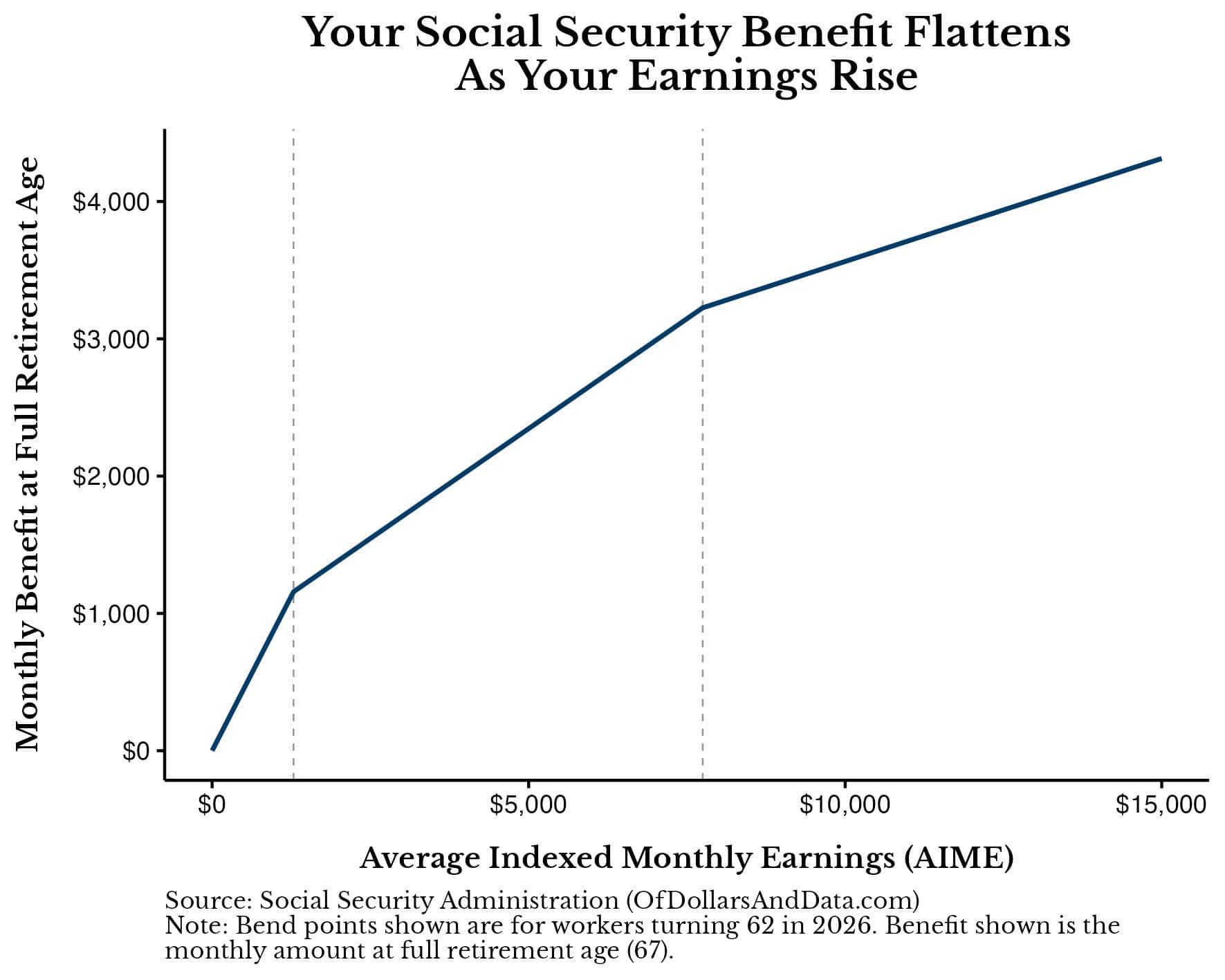
Monthly benefit against AIME. The slope flattens at the $1,286 and $7,749 bend points.1 / 2
A viral poll claiming that boomers back higher taxes on younger workers to protect their Social Security brought back an old question: can people in their 20s to 40s count on Social Security at all? Nick Maggiulli of Of Dollars and Data says yes, though not on all of it.
What "running out" means
Two trust funds pay benefits. The disability fund is projected to stay solvent through 2100. The retirement fund, 1 (Old-Age and Survivors Insurance), is not. It has been shrinking since 2021, the first year benefits paid out exceeded payroll taxes plus interest. The 2026 2 projects it will be empty in 2032. Money can't be moved between the two funds unless Congress passes a law.
Social Security can't borrow, so once OASI is empty it can only pay out what payroll taxes bring in. That covers about 78% of scheduled benefits at first, falling to about 62% by 2100 as the number of workers per retiree drops. Applied to today's average benefit of about $2,000 a month, 78% works out to roughly $1,560.
How your benefit is set
The Social Security Administration (SSA) takes three steps:
Index each year's earnings, up to that year's taxable cap ($184,500 in 2026), to national wage growth.
Average your 35 highest years. The total is always divided by 420 months, even if you worked fewer years. The result is your Average Indexed Monthly Earnings (3).
Apply "4." You get 90% of the first $1,286 of AIME, 32% of the amount up to $7,749, and 15% of anything above that.
The formula favors lower earners. For example, an AIME of $5,000 pays $2,345 a month at age 67, which is 46.9% of AIME. Claiming at 62 cuts that to about $1,642. Waiting until 70 raises it to about $2,908.
Fixing the gap
Congress can raise revenue or cut benefits. Measured against the 2025 shortfall:
Raising the payroll tax from 12.4% to 16.4% would close all of it.
Removing the earnings cap would close 67%.
Indexing bend points to prices instead of wages would close 74%.
Cutting the annual cost-of-living raise by one percentage point would close 51%.
Gradually raising the retirement age to 68 would close only 12%.
The 2026 shortfall is larger, so each option now closes a bit less. In a 2025 survey, 85% of respondents wanted benefits kept or increased, even if that meant higher taxes. Maggiulli expects tax increases to do most of the work.
Planning number
Maggiulli plans on 70% of his estimate from the SSA's my Social Security site. Here is his example:
A $3,000 estimate becomes $2,100 a month.
Against $8,000 of monthly spending, that leaves $5,900 a month, or $70,800 a year, to cover from savings.
At 25 times annual spending (the 5), that requires about $1.77 million.
His conclusion is that assuming Social Security won't exist is a bigger mistake than relying on it too heavily.
A widely shared poll, claiming that baby boomers overwhelmingly support higher taxes on younger workers to keep their Social Security benefits intact, prompted Nick Maggiulli of Of Dollars and Data to answer a question younger readers often ask him: can I count on Social Security in retirement? His answer is that the program will keep paying something, and he argues that planning on roughly 70% of your scheduled benefit is reasonable.
Two trust funds, one problem
Benefits come from two sources: payroll taxes on current workers and trust funds built up from past surpluses. There are actually two funds. The Disability Insurance (DI) fund pays disability benefits and is projected to pay in full through 2100, the end of the 75-year projection window. The Old-Age and Survivors Insurance (1) fund pays retirement and survivor benefits and is the one in trouble. The two are often quoted together as OASDI, but money can't move between them unless Congress passes a law. Maggiulli assumes that doesn't happen and looks at OASI alone.
OASI started drawing down in 2021. That was the first year retirement benefits exceeded the payroll taxes plus interest the fund collected, so it had to sell off principal. The 2026 2 projects the fund will be empty in 2032.
What happens then is often misunderstood. Social Security can't borrow, so after the fund is gone it must cut benefits to whatever incoming payroll taxes can pay for. That is about 78% of scheduled benefits in the first year, a 22% cut but not a 100% one. The share then falls as the number of workers per retiree keeps shrinking, reaching about 62% by 2100. For today's average benefit of about $2,000 a month, 78% means about $1,560.
How a benefit is calculated
Many people assume benefits work like a pension, where more years of work means a bigger payout. That is only true if income stays the same. The Social Security Administration (SSA) uses three steps.
1. Index earnings to wages. Each year's earnings are scaled up by growth in the national average wage index (3), measured up to the year you turn 60. Maggiulli earned $36,813 in 2012. The AWI rose 57.6% between 2012 and 2024 (69,846.57 ÷ 44,321.67), so that year counts as about $58,017 in 2024 terms. He uses 2024 for simplicity, since his actual index year, 2049, hasn't happened yet. Earnings above each year's taxable maximum are ignored. The cap is $184,500 in 2026 and was $110,100 in 2012.
2. Average the top 35 years. Add up your 35 highest indexed years and divide by 420, the number of months in 35 years. The result is your Average Indexed Monthly Earnings (4). You divide by 420 no matter how many years you worked. Ten years at the $184,500 cap and twenty years at half the cap both total $1,845,000, so both give an AIME of $4,392.86.
3. Apply the 5. For someone turning 62 in 2026, the benefit at full retirement age is:
90% of the first $1,286 of AIME
32% of the amount between $1,286 and $7,749
15% of the amount above $7,749
Maggiulli compares this to a marginal income tax schedule running in reverse: each slice of earnings is "paid back" at a lower rate than the slice before. The result is that low earners get most of their earnings replaced and high earners get a much smaller share.
Worked example (from the article): with an AIME of $5,000, the benefit is 0.9 × $1,286 + 0.32 × ($5,000 − $1,286) = about $2,345 a month at the full retirement age of 67. That is 46.9% of AIME. Claiming at 62 cuts it by about 30%, to $1,642. Waiting until 70 adds about 24%, for $2,908. The largest possible benefit in 2026 is $5,181 a month. It goes to people who earned at or above the cap for 35 or more years and waited until 70 to claim.
You can see your own projected benefits at 62, 67 and 70 on the SSA's "my Social Security" website.
The options for closing the gap
The SSA has estimated how much of the shortfall each proposed change would close. The figures below are measured against the 2025 shortfall. The 2026 shortfall is larger, so each would close somewhat less today.
The price-indexing option needs explaining. Wages usually grow faster than prices, and tying bend points to wages keeps benefits in step with living standards. Social Security has historically replaced about 40% of a median earner's wages. Tying the bend points to prices instead would gradually cut that share in half.
Raising the payroll tax is the only option on the list that closes the whole gap by itself. In a 2025 National Academy of Social Insurance survey, 85% of respondents said benefits should be kept or increased even if that meant raising taxes. Maggiulli therefore leans toward a future of higher taxes rather than smaller checks.
A planning rule
Maggiulli expects Congress to act in some way. Whether through a legislated fix or the fund running dry, he plans on receiving 70% of scheduled benefits. For the average person retiring in 2032, that is about $1,400 a month. He expects people retiring later to get more, even after inflation, because wages, and therefore AIME, tend to grow faster than prices.
His method:
Take your SSA estimate and multiply it by 0.7. A $3,000 estimate becomes $2,100.
Subtract that from your expected spending. With $8,000 a month in spending, savings must cover $5,900 a month, or $70,800 a year.
Multiply by 25 (the 7). That gives roughly $1.77 million needed on top of Social Security.
Caveats
Maggiulli admits nothing is guaranteed. Congress could change the program drastically, though he doesn't expect it to. The 70% figure is his own judgment, not a projection. The article also doesn't say how taxes on benefits, spousal benefits or future changes to the earnings cap would affect any individual's numbers. His bottom line is that you shouldn't build a retirement plan around the Social Security check, but assuming it won't come at all is the bigger mistake.
Remember
Once the fund is empty, payroll taxes alone still cover about 78% of benefits, falling to about 62% by 2100.
Benefits are averaged over 35 years and replace a shrinking share of income above each bend point.
Only raising the payroll tax to 16.4% closes the whole shortfall on its own; raising the retirement age to 68 closes 12%.
Year-over-year change in the Case-Shiller indices; the National index is now up 2.1%.1 / 3
S&P's 1 National Home Price Index rose 2.1% in the year to August 2026, up from 1.9% in July and a little above forecasts. Consumer prices rose 3.4% over the same year, so homes lost about 1.3 percentage points of value in 2 (inflation-adjusted) terms. It is the 15th straight month of real declines, though the gap is narrowing.
Read it as spring-to-summer data
Case-Shiller compares each home's sale price with its own previous sale. Its "August" figure is a three-month average of closings in June, July and August, and many June closings come from contracts signed in April. The release mostly reflects prices buyers agreed to months ago.
The big-city indices rose faster than the national one. The 20-City Composite was up 2.7% (from 2.5%), and the 10-City Composite was up 3.6% (from 3.4%).
Down on paper, up underneath
Before adjustment, the National index fell 0.2% from July. After 3 it rose 0.3%. Seasonal adjustment removes the usual pattern of prices peaking in summer and easing afterwards. So a raw dip in August is normal, and the adjusted gain means this August was stronger than a typical one. Rebecca Kaufman of S&P says the post-summer slowdown is "obscuring some underlying strength."
To make the real decline concrete, here is an illustrative example: a $400,000 home that rose 2.1% would be worth about $408,400 a year later. To keep up with 3.4% inflation it would need to be worth about $413,600.
A nine-point regional spread
Up most: Chicago +6.7% (top for six months running), New York +6.2%, Cleveland +4.3%
Down most: Seattle −2.0%, Las Vegas −1.3%, Denver −0.8%
The Midwest and Northeast are rising while parts of the West are falling. The national average hides very different local markets.
A second index agrees
The Federal Housing Finance Agency (4) runs its own index, built from mortgages backed by 5. It rose 0.3% in August and 2.4% over the year, and July's gain was revised down to 0.2%. The FHFA index also sets the 6, the largest mortgage those two companies will buy. Its regional figures ranged from +0.5% in the Mountain states to +4.4% in East North Central, which includes Chicago and Cleveland.
Still not affordable
Kaufman notes that buying remains hard. Mortgage rates are in the mid-to-high 6% range, inflation is 3.4% and oil is near $100 a barrel. The release doesn't explain why the regions have diverged so sharply, and Bill McBride's outlook section at Calculated Risk is behind a paywall.
S&P released its 1 home price indices for August 2026 on October 27. The National index rose 2.1% from a year earlier, up from 1.9% in July and above forecasts. Consumer prices rose 3.4% over the same year, though, so US home values fell in 2 (inflation-adjusted) terms for the 15th month in a row. Bill McBride of Calculated Risk set the release beside a second gauge, the Federal Housing Finance Agency (3) index, which showed a similar 2.4% annual gain.
What "August" actually means
The data runs well behind the calendar. Case-Shiller's "August" figure is a three-month average of closing prices from June, July and August. Many June closings come from contracts signed in April, because a home sale usually takes one to two months to close. So the release partly describes what buyers agreed to pay in the spring. That is worth keeping in mind before reading it as a sign of where the market is heading now.
The indices use the 4. Each home's sale price is compared with its own previous sale, which keeps the number from jumping just because more expensive homes happened to sell one month. The National index covers all nine US census divisions. The 10-City and 20-City Composites follow major metro areas.
The headline numbers
Year over year, not seasonally adjusted (5):
Index
Aug 2026
Jul 2026
National
+2.1%
+1.9%
20-City Composite
+2.7%
+2.5%
10-City Composite
+3.6%
+3.4%
All three sped up by about 0.2 percentage points. The big-city composites are rising faster than the national figure, which means prices outside the largest metros are rising more slowly.
Why the monthly numbers point in opposite directions
Before adjustment, the National index fell 0.2% from July, and the 10- and 20-City Composites each fell 0.4%. After 6, the National index rose 0.3% (0.28% to two decimals), the 10-City rose 0.4% and the 20-City rose 0.3%. McBride's own text gives the two composites' adjusted gains the other way round, but the direction is the same either way.
The gap comes from the calendar. Home prices usually peak in late spring and summer and soften once the selling season ends. A raw decline in August is normal. The adjusted figures ask a different question: was August better or worse than an ordinary August? The answer is better. Rebecca Kaufman of S&P Dow Jones Indices says the usual post-summer slowdown "is obscuring some underlying strength in home prices."
What "falling in real terms" means
An illustrative example, not taken from the article: a home worth $400,000 in August 2025 would be worth about $408,400 a year later after a 2.1% gain. To keep pace with 3.4% inflation it would need to reach about $413,600. The roughly $5,200 shortfall is the 1.3-percentage-point real loss S&P describes. Fifteen months of small losses like that add up, though S&P notes the gap has narrowed as nominal price growth picked up.
A nine-point spread between cities
Regional differences are large. The gap between the strongest and weakest metro areas is nearly 9 percentage points:
Strongest: Chicago +6.7% (top for the sixth month running), New York +6.2%, Cleveland +4.3%
Weakest: Seattle −2.0% (largest decline for the third month running), Las Vegas −1.3%, Denver −0.8%
Midwestern and Northeastern markets are leading. Western markets, many of which rose sharply earlier in the decade, are falling. The national average of 2.1% hides very different outcomes depending on where you live.
The second opinion: FHFA
The FHFA index rose 0.3% in August after seasonal adjustment and 2.4% from August 2025. July's gain was revised down from 0.3% to 0.2%. FHFA builds its index from mortgages bought or guaranteed by 7, the government-sponsored companies that buy most standard US home loans. That means it leaves out the jumbo loans and cash purchases that Case-Shiller includes. FHFA's index also has a practical use: it sets the 8, the largest mortgage Fannie and Freddie will buy. When prices rise, next year's limit rises with them.
FHFA's regional figures tell a similar story. Monthly changes ranged from −0.8% in New England to +2.1% in East South Central (Kentucky, Tennessee, Mississippi, Alabama). Over 12 months, the range ran from +0.5% in the Mountain division to +4.4% in East North Central, which includes Chicago and Cleveland. That fits Case-Shiller's metro leaders.
Affordability
Kaufman points out that even as prices lag inflation, buying a home is still hard. Inflation is at 3.4%, Brent crude oil is near $100 a barrel, and mortgage rates are in the mid-to-high 6% range. Prices that are flat in real terms do not make homes cheap when financing costs this much and household budgets are already stretched.
What's left open
The release doesn't say why the regions have split so sharply. Possible reasons include housing supply, local job markets, and how much each area rose earlier, but none of these are covered. It also doesn't say whether the faster nominal growth will last as autumn data arrives. McBride's "few things to watch" section, where he might weigh in, is behind a paywall. Because of the April-to-August lag, it will take a few more releases to see whether the summer's adjusted strength holds.
Remember
Case-Shiller's August figure averages June–August closings, partly reflecting contracts signed in April.
A raw monthly price drop in late summer is normal; the seasonally adjusted figure is the one to watch.
Local markets differ a lot: Chicago up 6.7%, Seattle down 2.0%, almost nine points apart.
New home sales since 1963 with recessions shaded; the current 676,000 pace is near pre-pandemic levels.1 / 3
The headline number
New single-family homes sold at a 1 of 676,000 in September 2026, according to the Census Bureau and the Department of Housing and Urban Development (2). A SAAR is a month's sales with normal seasonal swings removed, scaled up to a yearly pace.
That pace was 0.6% below August's 680,000 and 5.3% below September 2025's 714,000. It still beat the 660,000 forecasters expected, and the previous three months were revised up slightly. Bill McBride of Calculated Risk says sales are now close to pre-pandemic levels. Monthly estimates of new home sales are noisy and often revised, so the yearly trend tells you more than the small monthly dip.
Supply is still high
At the end of September, 476,000 new homes were for sale, down 2.3% from a year earlier. 3 measures how long that stock would last at the current sales pace:
676,000 a year ÷ 12 ≈ 56,300 sales a month
476,000 ÷ 56,300 ≈ 8.4 months
That is down slightly from 8.5 months in August but up from 8.2 a year ago. Inventory fell over the year, but sales fell faster. A balanced market usually has 4 to 6 months of supply. The record high was 12.2 months in January 2009 and the record low was 3.3 months in August 2020.
What "for sale" includes
The Census Bureau counts a house as for sale once a building permit is issued and no contract or deposit has been taken. So inventory includes homes that don't physically exist yet. It splits the total three ways:
4: 111,000. More than triple the February 2022 low of 31,000 and above normal, but down from 128,000 in January 2026.
Under construction: 250,000. High, but 22% below its cycle peak.
5: 115,000. An all-time high.
Finished, unsold homes cost builders the most, because the money is already spent and carrying costs keep running. The drop since January suggests builders have been clearing that stock. The article doesn't say why not-started inventory is at a record. One possibility is that builders are holding permits and waiting for buyers before breaking ground.
Overall, sales are steady, supply is well above normal, and builders are trimming finished inventory. The free part of the post doesn't cover prices, regional detail, or its seasonal comparison chart. Those are for paid subscribers.
The September numbers
The U.S. Census Bureau and the Department of Housing and Urban Development (1) report that new single-family homes sold at a 2 of 676,000 in September 2026. A SAAR is the month's sales with normal seasonal swings removed, scaled up to a yearly pace. The figure is 0.6% below August's 680,000 and 5.3% below the 714,000 pace of September 2025.
Forecasters had expected 660,000, so the result beat the 3. Sales for the previous three months were also revised up slightly when taken together. Bill McBride of Calculated Risk notes that sales are now close to their pre-pandemic level. His first chart plots new home sales against recessions back to 1963.
The revisions matter. New home sales come from a survey of a fairly small sample, and monthly estimates often get revised by a meaningful amount. A 0.6% monthly drop is within the noise. The year-over-year decline and the inventory trend tell you more.
How much supply is sitting unsold
At the end of September, 476,000 new houses were for sale (seasonally adjusted). That is 1.0% below August's 481,000 and 2.3% below the 487,000 of a year earlier.
4 converts that inventory into time. Here is the arithmetic:
676,000 a year ÷ 12 ≈ 56,300 homes sold per month
476,000 for sale ÷ 56,300 ≈ 8.4 months
So if builders stopped adding homes, current stock would take about 8.4 months to sell at September's pace. That is down from 8.5 months in August but up 2.4% from 8.2 months a year ago. Inventory fell over the year, but sales fell faster, so the supply measure rose.
For scale:
Normal: about 4 to 6 months
Record high: 12.2 months, in January 2009, during the housing bust
Record low: 3.3 months, in August 2020, during the pandemic buying rush
At 8.4 months, McBride says, supply is "well above the top of the normal range."
Three kinds of inventory
How the Census Bureau defines "for sale" matters. A house counts as for sale once a building permit has been issued (or, where no permit is needed, once work has started on the foundation), as long as no sales contract has been signed and no deposit taken. So the 476,000 figure includes many homes that are only permits on a lot.
Since 1973 the Bureau has split inventory into three groups, shown in McBride's third chart:
5 (111,000): finished homes waiting for a buyer. That is more than triple the record low of 31,000 in February 2022 and above the normal level, though below the recent peak of 128,000 in January 2026.
Under construction (250,000): described as high but 22% below its cycle peak.
6 (115,000): permitted but not yet begun. This is an all-time high.
The groups carry different risks for builders. A completed, unsold home is the expensive kind of inventory: the builder has spent the money on land, materials and labour and pays interest and upkeep until it sells. Builders usually work that stock down with price cuts or incentives such as paying to lower a buyer's mortgage rate. (That is general industry practice; the article doesn't discuss pricing.) Completed inventory falling from its January peak suggests builders have been clearing some of it.
A record number of not-started homes is harder to read, and the article doesn't interpret it. One possibility is that builders have permits in hand but are waiting for contracts before they break ground, which limits their exposure if demand weakens. Another is that permits were pulled during a more optimistic period. Either way, those homes add to measured supply without yet being physical houses.
What the picture adds up to
Taken together: sales are steady at roughly pre-pandemic levels and slightly better than expected. They are down from a year ago, and supply is well above normal. Builders appear to be trimming the costliest inventory (completed homes) and the pipeline under construction, while not-started inventory reaches a record. A high months-of-supply figure usually points to softer new-home prices and fewer housing starts ahead. The article itself doesn't make that forecast.
What the article leaves out
The free part of the post doesn't cover prices, regional splits, or McBride's fourth chart, which compares not-seasonally-adjusted monthly sales for 2019 to 2026 against the 2005 bubble peak and the 2008 to 2011 bust lows. That analysis is for paid subscribers. It also doesn't say what drove the consensus beat or how mortgage rates figured into September demand.
Remember
Months of supply rose over the year because sales fell faster than inventory, even though inventory itself shrank.
Census counts permitted, unbuilt homes as inventory; 115,000 'not started' homes is a record.
Completed unsold homes are down from January's 128,000 peak but still more than triple the 2022 low.
Third markets are countries outside both China and the EU. Comparing market share there shows who wins head-to-head competition for the same customers, without the distortion of home-market loyalty or tariffs between China and the EU.
Kiel Institute data: EU exporters lost third-market share to China across nearly all product groups, 2012–14 to 2022–24.1 / 2
European manufacturers and politicians are now preoccupied with what is being called the 1: Chinese companies competing with European firms in high-tech goods, both in Europe and in other countries. Joachim Klement, an investment strategist who writes the Klement on Investing newsletter, uses new research to argue that Germany is being hit hardest, and that price is not the main reason.
What the data shows
Economists at the 2, a German economic research institute (Chowdhry et al., 2026), compared exporters' 3 in 4, meaning countries outside both China and the EU. They looked at the change between the 2012–14 average and the 2022–24 average.
Across nearly every product category, EU manufacturers lost market share in those countries and Chinese manufacturers gained it. Leather goods, art and weapons were the only notable exceptions, and most of the leather goods are luxury items such as handbags. Over the same decade, Chinese exports to these markets also grew much faster than European ones.
Germany falls behind the European average
The researchers then asked whether each EU country lost share in proportion to the European average, or more than that. Germany lost more, and over a wide range of products. Its biggest "excess" losses came in its traditional strengths:
cars
machinery
electrical equipment
optical and medical equipment
Klement's post doesn't give the size of these losses. The figures appear only in the study's charts.
Klement's reading
The authors conclude, and Klement largely agrees, that Chinese goods have overtaken German output in quality and innovation as well as in price. Klement says many German manufacturers still deny this.
His conclusion is that 5 won't save companies that aren't innovative enough. A tariff can make Chinese goods dearer at home, but in third markets it does nothing. What German firms need, he says, is heavy investment in future technologies, and he points to the German car industry as evidence that this isn't happening.
Caveats
Losing market share doesn't necessarily mean shrinking: German exports could still grow in absolute terms while China's grow faster. The post also offers no direct evidence of Chinese quality, such as patents or reliability data. The quality argument is an inference from how widespread the share losses are. Klement's criticism of the car industry's investment is his own judgment, not a finding of the study.
Among European manufacturers and policymakers, the "1" is now a top concern. The term describes Chinese companies competing with European manufacturers in high-tech goods, both in Europe and in other countries. In a short post, Joachim Klement, an investment strategist who writes the Klement on Investing newsletter, uses new research from the 2, a German economic research institute, to argue two things. Germany is losing ground faster than the rest of Europe, and the underlying problem is quality and innovation, not just price.
Why this shock is different
The 3 in the 2000s was mostly about low-cost goods such as furniture, textiles and simple electronics. It displaced manufacturing workers in rich countries, but countries like Germany came out fairly well. German firms sold China the machine tools, cars and industrial equipment it needed to build its factories. The second shock reverses that: Chinese producers now compete directly in those same advanced categories.
Measuring this competition is harder than it looks. A firm's share of its own home market reflects 4, subsidies, brand loyalty and government purchasing. A cleaner test is 5, countries outside both China and the EU, where Chinese and European exporters sell to the same customers under broadly similar conditions. Rising Chinese share there means buyers are choosing Chinese goods on their merits.
Step one: Europe as a whole
The Kiel researchers (Chowdhry et al., 2026) calculated how Chinese and EU exporters' shares of third markets changed between the 2012–14 average and the 2022–24 average. Averaging over three years smooths out one-off swings in individual years.
The results are one-sided. Across nearly every product category, EU manufacturers lost share and Chinese manufacturers gained it. The few exceptions where Europe held up were leather goods (largely luxury items such as handbags), art and weapons. In those categories, brand, provenance or political alignment count for more than cost or technical specification.
The researchers also expressed the shift in growth terms: Chinese exports to these markets grew much faster than European exports over the decade. Klement's post doesn't give the headline figures. They appear only in the study's charts.
Step two: Germany against its peers
Next, the researchers tested whether every EU country lost share at the same rate. They compared Germany's actual change in each product category with the change it would have seen if it had moved exactly in line with the European average. The gap between the two is the "excess" loss or gain.
A simple illustration, with invented numbers: suppose EU exporters together lost 10% of their share in a product's third-market sales. If Germany's share in that product fell 10%, it simply moved with Europe. If it fell 18%, the extra 8 points is the excess, a loss specific to Germany.
Germany's results were bad. Its excess losses were large and covered many categories, and they were concentrated in the industries that define the German economy:
motor vehicles
machinery
electrical equipment
optical and medical equipment
These are exactly the categories where Germany has historically competed on engineering quality rather than price. Klement's post doesn't report the actual percentages.
The argument: quality, not just cost
The authors argue, and Klement says he largely agrees, that the breadth and location of the losses point to one conclusion. Chinese goods are no longer winning only on price. They now match or beat German products on quality and innovation. Klement adds that many German manufacturers still deny this.
The reasoning goes as follows. If the problem were only cost, such as Germany's high energy prices after 2022 or its labour costs, you would expect losses to concentrate in price-sensitive, commoditised goods. Instead they cluster in premium engineered products, where buyers have long been willing to pay more for German quality. When buyers stop paying that premium, the most likely explanation is that the quality gap has closed.
Why tariffs don't fix it
Klement's policy conclusion is that tariffs won't help manufacturers that aren't innovative enough. The third-market data shows why. An EU tariff on Chinese cars or machinery can protect sales inside Europe, but it does nothing in Brazil, Turkey, Southeast Asia or the Middle East, where German firms have to compete without protection. For an export-led economy like Germany's, those markets matter a great deal.
His alternative is heavy investment in future technologies. He cites the German car industry as evidence that this is not happening, though the post doesn't detail which investments he considers missing.
What the post leaves open
The evidence is suggestive but limited, and a careful reader should keep a few points in mind:
Share is not volume. Losing 6 doesn't necessarily mean shrinking. German exports to third markets could have grown in absolute terms while China's grew faster. The post doesn't say which happened.
Quality is inferred, not measured. The post presents no direct evidence on product quality, such as patents, reliability data or price premiums. The quality argument rests on where the share losses fall.
Other explanations exist. Chinese state subsidies, exchange-rate moves, Germany's energy-cost shock and German firms moving production abroad could each explain some of the pattern. The post doesn't weigh them.
Even with those limits, the core finding is notable. Over a decade, in the markets where competition is fairest, Germany has lost ground faster than its European neighbours, and it has lost most in the products that built its export strength.
Remember
Excluding luxury leather goods, art and weapons, EU exporters lost third-market share to China across nearly all products in 2012–24.
Germany's losses exceeded the European average most in cars, machinery, electrical, optical and medical equipment.
Tariffs protect home markets only, so they can't help German exporters compete in third countries.
1, Holmes's blood-testing startup, said it could run many diagnostic tests from a fingerprick of blood. It couldn't. When Vice President Joe Biden toured the company in 2015 and called it "the laboratory of the future," the lab was staged, the devices didn't work, and most staff had been told to stay home.
Rich investors still poured money in:
The Walton family (Walmart heirs) lost $150 million.
Rupert Murdoch put in $125 million on gut feel, then sold the stake for $1 to claim a 2.
Betsy DeVos's family lost $100 million.
A hedge fund bought shares at a price valuing the company at $9 billion, which made Holmes worth $5 billion on paper.
Two mechanisms: 3 and overconfidence
Carlson says investors didn't suspect anything because of who else was involved. The board included Henry Kissinger, George Shultz, Jim Mattis and William Perry. This is herding, or copying what others do. Each investor took the famous names as proof the company had been vetted. Nobody had actually checked that the product worked.
The second mechanism is personalizing success. Carlson cites Jim Paul, a commodities trader who made a fortune young and then lost it. Paul came to treat his wins as proof of his ability rather than of timing or luck. Success, Carlson argues, makes people feel invincible, and people around them stop holding them accountable.
The research
Carlson cites work by Richard West, Russell Meserve and Keith Stanovich on 4, the tendency to spot bias in others more easily than in yourself. Across seven measures of cognitive ability, they found that being smarter didn't reduce this blind spot. People who knew about their own biases weren't any better at overcoming them. Carlson adds that smarter people may simply be better at talking themselves into things.
How much weight to give it
This is a persuasive essay built on one dramatic case and one line of research. It doesn't show that wealthy investors make mistakes more often than anyone else. The most useful point is the study's: knowing about a bias doesn't fix it. That argues for outside checks, like verifying claims yourself and asking whether a past win was skill or luck. Carlson diagnoses the problem but offers no checklist.
Ben Carlson, a wealth manager who writes the blog A Wealth of Common Sense, has reposted an edited chapter from his book Don't Fall For It. The trigger, he says, is the attention around Nathan Fielder's new film about Elizabeth Holmes, You Can See Everything. His case is simple. Being smart and successful doesn't protect you from bad money decisions and can make them more likely. He thinks it's worth repeating now because confidence tends to rise along with markets in boom times.
The problem: smart people get taken too
Carlson opens with a line from the economist John Kenneth Galbraith: fools are "soon or eventually" separated from their money. Carlson's reply is that fools aren't the only ones. A high income, a large portfolio, a degree from a prestigious university or an impressive job title doesn't make you good at managing money. He argues that many of the worst investors are very successful in other fields.
1 as the case study
Theranos was Holmes's Silicon Valley blood-testing company. It promised to run a series of diagnostic tests from a pinprick of blood. Holmes dropped out of Stanford at 19 to build the device, which she called "the most important thing humanity has ever built."
Carlson describes how staged the company was. In 2015 Vice President Joe Biden toured the facilities and afterward called it "the laboratory of the future." The lab he saw was staged, the devices didn't work, and most lab workers had been told to stay home that day. Holmes also spoke in a deliberately deeper voice so she would sound more serious.
The losses Carlson lists:
The Walton family (heirs to the Walmart fortune): $150 million.
Rupert Murdoch: $125 million, invested on gut feel alone. He later sold the whole stake for $1 so he could claim a 2 on a worthless investment.
Betsy DeVos and her family: $100 million.
Other investors included Patriots owner Robert Kraft, Mexican billionaire Carlos Slim and a Greek shipping magnate.
Partner Fund Management, a well-known hedge fund, bought shares at a price that valued Theranos at $9 billion. On paper, that made Holmes worth $5 billion.
How it worked: borrowed credibility
Carlson argues that investors suspected nothing because of who else was involved. The board included former Defense Secretaries Jim Mattis and William Perry, former Secretaries of State George Shultz and Henry Kissinger, and retired Navy Admiral Gary Roughead. Shultz called Holmes "the next Steve Jobs or Bill Gates."
This is the 3 Carlson warns about. Each wealthy investor treated the other famous names as proof that someone had already checked the company. In fact, nobody had checked whether the devices worked. Status stood in for 4 (actually verifying the claims).
Why success breeds overconfidence
Carlson's second mechanism is "personalizing" success. He draws on Brendan Moynihan's book What I Learned Losing a Million Dollars, about Jim Paul. Paul made a fortune trading commodities when he was young, then lost it after the windfall went to his head. Moynihan's lesson is that people who treat their successes as proof of their own ability, rather than of a good opportunity, good timing or plain luck, start to believe their involvement guarantees success.
Carlson adds a social piece. When the people around you assume intelligence is all that matters, nobody holds you accountable for your decisions.
The evidence: 5
The one piece of research in the argument comes from Richard West, Russell Meserve and Keith Stanovich. They studied blind spot bias, the tendency to see bias in others more easily than in yourself. After testing seven measures of cognitive ability, they concluded that "cognitive ability did not attenuate this 6 bias." Metacognitive here means thinking about your own thinking. Being smarter didn't shrink the blind spot. They also found that "people who were aware of their own biases were not better able to overcome them."
Carlson goes further than that. He says the bias blind spot was actually bigger among people with higher cognitive ability. His explanation is that intelligent people have more mental firepower to talk themselves into things.
How much weight to put on this
The argument is mostly anecdote plus one line of research. Theranos is a striking example, but it was a private company sold to a small circle of very rich people. Carlson doesn't show that wealthy investors make mistakes more often than ordinary ones, only that they clearly make them. The study supports a narrower claim than "smart people are worse investors": intelligence doesn't protect you from a blind spot about your own biases, and simply knowing about biases doesn't fix them.
That second finding is the most useful one for an ordinary investor. If knowing about a bias doesn't cure it, then good intentions won't either. What helps are outside checks: verifying claims yourself instead of leaning on endorsements, and asking whether a past win was skill or luck. Carlson's chapter diagnoses the problem but offers no checklist. He doesn't say how to tell a real opportunity from a well-credentialed fraud, beyond implying that famous names are not evidence.
Remember
Famous backers and board members are not evidence. At Theranos, nobody had checked that the device worked.
Research suggests knowing about your biases doesn't help you overcome them. Outside checks work better than good intentions.
Big early wins can feel like proof of skill when they were really timing or luck.