Banks Die on Fridays, by Appointment · Morning Gist
Tuesday, November 35 stories · 16 min
Banks Die on Fridays, by Appointment
Supervisors shape when banks fail, insiders' timing looks empty, housing inventory rebuilds as prices barely rise, and an $850,000 gene therapy gets a financing argument.
Picked from 65 new articles across 16 sources · arrow keys for other days
Today in 30 seconds
30s left
All but 28 of 557 US commercial bank failures since 2000 came on a Friday, the day regulators prefer for closures. story 1 ↓
Across 47,458 insider purchases, stocks beat the typical stock but trailed the S&P 500; shifting purchases six months later kept the edge. story 2 ↓
US single-family listings are back at 2019 levels, up 6.8% from a year ago, with 30-year mortgage rates at 7.27%. story 3 ↓
Freddie Mac says home prices rose 1.9% in a year, but 20 states, D.C. and 151 of 387 metros trail peaks. story 4 ↓
Alex Tabarrok argues an $850,000 gene therapy price reflects one-time-cure economics, proposing instalment payments and lighter regulation over price controls. story 5 ↓
Two economists studying California's proposed billionaire tax reached sharply different conclusions on whether it would fill or drain state coffers.
1/5Liberty Street Economics (NY Fed)· Sergio Correia, Stephan Luck, and Emil Verner· Nov 2
Most US bank failures are supervisors' decisions, driven by numbers they help shape
Fed and MIT economists studied every commercial bank examination from 2000 to 2023. Supervisors usually close banks when reported capital collapses, but examiners also push banks to admit losses, and stricter oversight cuts closure costs while reducing lending.
Why it matters · When a bank's capital figure can decide its survival, how hard examiners push on losses affects taxpayers' and the insurance fund's bills, and how much credit reaches borrowers during a downturn.
Know this first
Context from the editor, not the article · 31 sec
1 · How banks get closed
A US bank does not normally go bankrupt in court. Its chartering authority closes it, and the Federal Deposit Insurance Corporation usually sells it to a healthier bank, protecting insured deposits of up to $250,000 per depositor, per bank.
2 · Thin capital cushions
Book equity is assets minus liabilities as recorded in a bank's accounts. Banks are highly leveraged, so equity is a small slice of assets, and recognizing a loan loss sooner or later can visibly move the ratio.
3 · Why depositors stay calm
2/5HumbleDollar· Daniel Oliveira· Nov 3
Insider stock purchases beat the typical stock but trailed the S&P 500
A data firm measured 47,458 executive stock purchases from 2020 to 2025. A year later they slightly beat the typical stock but lagged the S&P 500 by about 13 points, and their timing added nothing.
Why it matters · Headlines treat insider buying as a tip, but for someone who owns an index fund, this data suggests it points to a company type, not a reason to act.
Know this first
Context from the editor, not the article · 20 sec
1 · What insider buying is
Company officers, directors and large shareholders must report their trades in its stock to the U.S. securities regulator, usually within two business days. That makes their purchases public, and financial news often reports them as a vote of confidence.
2 · Median versus index return
The median stock is the one in the middle of the pack, regardless of size. The S&P 500 weights companies by market value, so a few giants can lift it far above what the typical stock earns.
Image: HumbleDollar
3/5Calculated Risk· CalculatedRisk by Bill McBride· Nov 2
US single-family home listings return to 2019 levels as buyers pull back
Housing analyst Bill McBride reports that single-family homes for sale have matched 2019 levels for the first time in this cycle's data shown. Weak demand is driving the rise, and he expects slower sales and pressure on prices.
Why it matters · Listings often shift before prices do, so this gives buyers and sellers an early read on bargaining power, without waiting for sales and price reports that arrive later.
Know this first
Context from the editor, not the article · 28 sec
1 · Why 2019 is the benchmark
Homes for sale fell sharply during the pandemic as low mortgage rates pulled in buyers. Analysts often compare today's market with 2019, the last full year before that disruption, as a rough stand-in for normal.
2 · Inventory is a stock
Inventory counts the homes listed at one moment. New listings add to it; sales and withdrawn listings subtract from it. So it can rise because fewer homes are selling, even if no more owners decide to sell.
3 · Mortgage rates set affordability
Most US buyers borrow with a fixed-rate 30-year mortgage, so the rate largely determines the monthly payment they can afford. When rates are high, the same budget supports a smaller loan and demand tends to weaken.
4/5Calculated Risk· CalculatedRisk by Bill McBride· Nov 2
US home prices up 1.9% from a year ago, Freddie Mac reports
Freddie Mac's national home price index rose 0.15% in September and 1.9% over the year. Analyst Bill McBride expects annual growth to slow, while many Florida and Texas cities remain well below their peaks.
Why it matters · Home prices drive household wealth and buying decisions, and this reading shows why a modest national figure can hide meaningful losses for owners in particular markets.
Know this first
Context from the editor, not the article · 27 sec
1 · Repeat-sales price indexes
These indexes track price changes in the same homes over time, comparing each sale with that home's earlier value. This reduces distortion from the mix of homes sold, which can swing simple median prices.
2 · Fannie Mae and Freddie Mac
These two government-sponsored companies buy mortgages from lenders and package them into securities. Because they see so many loans, their data can power a price index, though it covers only mortgages they purchase.
3 · Monthly and annual changes
Monthly changes show recent momentum but can be noisy, so they are usually adjusted for seasonal patterns. Annual changes are steadier, but they also depend on what prices did during the same months a year earlier.
5/5Marginal Revolution· Alex Tabarrok· Nov 2
Economist argues $850,000 gene therapy price reflects drug economics, not just profiteering
Economist Alex Tabarrok argues Luxturna's $850,000 price reflects failed drug projects, one-time cures and tiny patient groups. He favors paying over time and cutting development costs rather than simply capping prices.
Why it matters · More drugs will treat small groups or cure with one dose, so who pays, when and how much will increasingly shape insurance costs and patient access.
Know this first
Context from the editor, not the article · 29 sec
1 · How drugmakers recoup research
Developing a drug costs far more than manufacturing it, and most candidates fail in testing. Patents and regulatory exclusivity give successful drugs a limited period of protected pricing, which is when companies try to earn back research spending.
2 · What Luxturna is
Luxturna, approved in the US in 2017, treats vision loss caused by mutations in both copies of the RPE65 gene. It is injected once into each eye, with a list price of $425,000 per eye.
3 · Why cures strain insurance
Insurers usually pay for chronic treatment gradually, month by month. A one-time therapy brings the whole bill forward, and in the US the patient may later change insurers, so the original payer may not capture the long-term benefits.
Insured depositors get their money back even if a bank fails, so they have little reason to monitor it or rush out. Deposit insurance prevents many runs, but it also removes a warning signal and leaves more of the policing to government supervisors.
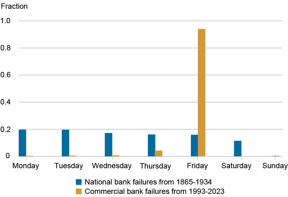
Failures spread evenly across weekdays before federal deposit insurance, but cluster overwhelmingly on Fridays in the modern era.1 / 4
US banks rarely fail the way they do in old photographs, with crowds at the door. A study of all commercial bank examinations from 2000 to 2023, by economists at the Richmond Fed, New York Fed and MIT, finds that failure is usually a supervisor's decision, based on a capital number supervisors help shape.
The Friday test
Of 557 commercial bank failures since 2000, only 28 happened on a day other than Friday, the preferred closure day of the 1 (FDIC), the US deposit insurer. Another bank typically buys the failed one in a deal arranged in advance. Between 1865 and 1935, failures were spread about evenly across weekdays, suggesting owners or depositors largely set the timing.
The authors link this shift to deposit insurance. Insured depositors have less reason to run, so supervisors partly take over the job of disciplining weak banks.
The number that matters
Closure closely tracks 2, a bank's recorded assets minus liabilities, as a share of its assets:
Above 5 percent: banks effectively never fail within a year.
Below 5 percent: closure risk climbs quickly.
Below 2 percent: closure risk reaches almost 70 percent.
Supervisors' confidential 3 ratings, which grade banks from 1 (strong) to 5 (critically deficient), follow the same figure when banks are weak. Banks under 4 percent almost always get a 4 or 5. Examiners appear to use more judgment with well-capitalized banks.
Examiners help write the number
Banks report their finances in quarterly filings called 4, which they can later revise. The chance of a revision to income or equity jumps during an on-site examination and in the two months after it. That suggests examinations push banks to admit losses they had not yet reported.
Single revisions are small, but they accumulate. The typical failing bank's equity ratio falls 8 percentage points in its last five years, and nearly 3 of those points come from revisions. So the hard number that drives closure is partly a product of supervision.
The trade-off
During the 2008 crisis, otherwise similar banks were quasi-randomly assigned stricter supervisors, those who gave worse ratings for the same financial condition. That made it possible to measure cause and effect. Banks with stricter supervisors recognized more losses, reported less equity and were more likely to fail. Failures cost the FDIC less, but credit fell in the short term.
Strictness limits 5, which survive while misallocating credit, and 6, where near-insolvent banks take big risks at the insurer's expense. 7, or holding off on tough action, can preserve lending and let banks recover if asset values improve.
The authors decline to say how strict supervisors should be, and this summary doesn't give the size of the cost savings or the credit decline.
Three economists, Sergio Correia of the Richmond Fed, Stephan Luck of the New York Fed and Emil Verner of MIT, have examined how US supervisors handle failing banks, using data on all commercial bank examinations from 2000 to 2023. In a staff report summarized on the New York Fed's Liberty Street Economics blog, they find that a modern bank failure is usually a supervisory decision, triggered by low reported capital. That capital figure, however, is partly a product of supervision itself.
The problem supervisors are solving
The authors give supervision two jobs with distressed banks. The first is producing information: verifying financial statements, forcing out hidden losses, and judging loan quality and management. The second is discipline: making a weak bank recognize losses, raise capital or close.
These jobs matter more because of deposit insurance. Insured depositors have little reason to watch their bank, so the market signal that once came from withdrawals has weakened. The hard part is timing. Close a bank too late and its losses can grow. Act too early and you may kill a bank that could have recovered, and cut lending when borrowers need it most.
Failures moved to Fridays
The clearest evidence is the calendar. Of the 557 commercial bank failures since 2000, only 28 happened on a day other than Friday, the preferred closure day of the 1 (FDIC), the US deposit insurer and usual manager of failed banks. Failed banks are almost always bought by another bank, typically in a deal arranged before the formal failure.
Between 1865 and 1935, by contrast, national bank failures were spread about evenly across weekdays. The authors read this as a sign that owners or depositors then largely set the timing. Today's Friday pattern suggests that failure now follows an official's schedule, not a panic's, though the authors note "notable exceptions," which they don't name. Silicon Valley Bank, closed amid a deposit run in 2023, is a well-known recent example.
A hard number drives closure
Supervisors act on what the authors call 2, meaning verifiable figures rather than judgment calls. The key one is 3, the accounting value of assets minus liabilities, as a share of assets.
Above a 5 percent ratio, banks effectively never fail within the following year.
Below 5 percent, the probability of closure rises quickly as capital falls.
Below 2 percent, it reaches almost 70 percent.
The post doesn't spell out the legal backdrop, but it helps explain the pattern. Under 4, a US framework dating from 1991, regulators must escalate restrictions as capital falls. A bank whose tangible equity drops to 2 percent is classed as critically undercapitalized and generally must enter receivership within 90 days.
Supervisory ratings show a similar link. 5 scores, confidential grades from 1 (strong) to 5 (critically deficient), cover capital, assets, management, earnings, liquidity and sensitivity to market risk. Banks above a 7.5 percent ratio are typically rated 1 or 2, averaging about 1.8. Those under 4 percent almost always get a 4 or 5, and their average is well above 4.
The components are revealing. For poorly capitalized banks, the composite score nearly matches the capital score, leaving little apparent room for judgment. For well-capitalized banks, the composite sits above the capital score, meaning worse, and closer to the management score. The authors read that as supervisors using discretion mainly when a bank isn't in distress.
One caution on these figures: the text speaks of equity-to-assets, while the chart notes use the 6 (CET1) ratio, which divides core capital by risk-weighted assets. The two measures aren't identical, so treat the thresholds as approximate guides rather than legal lines.
The hard number is partly made by examiners
Banks file quarterly financial statements called 7, and they can later revise them. The authors track revisions to net income or book equity around on-site examinations, using a 2007–23 sample. The chance of a revision rises slightly in the two months before an exam, then jumps in the exam month and the following two months. That timing suggests that examinations prompt banks to change what they first reported, though the chart alone shows association rather than proof of an examiner's demand.
Any single revision is small, but they add up for failing banks. In the five years before failure, the typical failing bank's equity-to-assets ratio falls 8 percentage points, and revisions account for nearly 3 of those points.
An illustrative example, with invented starting numbers and assets held constant: a bank with $1 billion in assets and $90 million in equity has a 9 percent ratio. An 8-point decline takes equity to $10 million, or 1 percent. If $30 million of that came through revisions, the bank's original filings alone would show 4 percent. That places it in the elevated-risk zone, but not below the 2 percent mark where failure is close to 70 percent likely. This doesn't mean the bank would otherwise have survived, since revisions may simply bring forward losses that were coming anyway. It shows why a closure rule based on hard data still leaves supervisors with considerable influence.
What strictness costs and buys
To test cause and effect, the authors use a natural experiment from the 2008 financial crisis, in which otherwise similar banks were quasi-randomly assigned stricter supervisors. A "stricter" supervisor is one who gives a worse CAMELS rating for the same financial condition. The post doesn't describe how this assignment worked; that detail is in the full paper.
Stricter supervision made banks recognize more losses and report less equity, which raised their likelihood of failure. It also lowered failure costs for the FDIC, but reduced credit in the short term. The post doesn't give the sizes of these effects.
Each choice has a recognizable risk. Strictness limits 8, where a nearly insolvent bank takes big risks because its owners keep any gains while losses fall on the insurer. It also limits 9, which stay open and keep misallocating credit. 10, or holding off on tough action, can preserve lending and give a bank time to recover if its assets regain value. But if they don't, the eventual bill may be larger.
What remains open
The authors explicitly decline to say how strict supervisors should be. Their analysis describes effects without recommending a policy. The natural experiment also comes from one severe crisis, and the post doesn't say whether its results would hold in a milder downturn. Short-term credit losses and lower resolution costs also aren't measured in a common unit here, so the post alone can't tell a reader which side of the trade-off is larger.
Remember
Friday closures are a fingerprint: failure timing moved from depositors and owners to the FDIC's schedule.
A rule based on reported capital still leaves room for judgment, because examiners influence what gets reported.
Forcing losses into the open early can lower closure costs while shrinking credit when borrowers most need it.
News that an executive bought shares in their own company often reads like a tip. Daniel Oliveira, who works at the data firm Equibles, tested that idea on 47,458 insider 1, meaning shares bought on the exchange rather than received as pay, in American stocks from January 2020 to August 2025.
The answer depends on the yardstick
A year after the purchase, the typical stock was up 2.36%. Two comparisons give opposite verdicts:
Against the 2 listed stock: purchases led by 2.56 3, and 53% beat it.
Against the 4, an index of large U.S. companies weighted by market value: purchases trailed by 12.95 points, and only 37% beat it.
The gap exists because insiders mostly buy small companies. Over these years the median stock went nowhere, while the S&P 500 returned 17.84% over a typical one-year window.
Timing added nothing
If insiders knew good news was coming, the edge should sit close to the purchase date. To test this, the study moved each purchase's one-year window six months later, as if the insider had bought long afterwards.
The lead over the median stock did not shrink: it was 2.78% for the shifted dates and 2.61% for the real ones. Oliveira's conclusion is that insider buying "marks a type of company, not a moment." In other words, the small lead appears to belong to the kinds of firms insiders buy, whenever you happen to hold them.
Stronger-looking signals did worse
Two signals that sound especially convincing also failed:
Big purchases: the largest tenth, with a median size of $3.53 million, trailed the smallest tenth by 17.1 points over a year.
A first purchase after two quiet years: 858 of these returned a median 0.74% over the next year, while the median S&P 500 member returned 7.50%.
What to make of it
Oliveira's lesson for index fund investors is about the 5: the same purchases look like a win against the typical stock and a loss against the index most people own.
Some caution is due. This is a short summary by an employee of the firm behind the study, and it covers one period in which large companies did unusually well. The figures are medians, so they don't show what a portfolio of these stocks would have earned, and the post reports no adjustment for risk or trading costs.
It also reports only one-year results, so it says nothing about whether insiders' purchases predict returns over shorter periods. The finding is best read as evidence against treating a purchase headline as a reason to act, not as proof that insiders know nothing.
Daniel Oliveira, who works at the data firm Equibles, has published a test of a familiar market story: that an executive buying shares in their own company is effectively a tip. Equibles measured what followed 47,458 insider 1 of American stocks from January 2020 to August 2025. These are purchases made on the exchange with the insider's own money, as opposed to shares received as pay. The data comes from filings with the 2, the U.S. markets regulator, combined with daily prices.
The short version is that the result flips depending on what you compare it with, and the timing of the purchases seems to carry no information.
Why this is hard to measure
A raw return says little by itself. The typical purchase was followed by a 2.36% gain over a year, which only means something next to a 3, the alternative an investor could have held instead. Insiders also don't buy a random sample of the market. They mostly buy small companies, so any comparison partly measures how small companies did relative to large ones, not what the insider knew.
Two benchmarks, opposite verdicts
Measured over the same windows, the purchases compare like this:
Benchmark
Purchases' lead or lag, one year
Share of purchases that beat it
Median listed stock
+2.56 points
53%
4
The 5 stock is the one in the middle of the market, with size ignored. The S&P 500 is an index of large U.S. companies weighted by market value, so its biggest members count most. Over these years the median stock went nowhere, while the S&P 500 returned 17.84% over a typical one-year window.
Even the favorable result is modest: 53% is only slightly better than a coin flip. The figures also don't subtract neatly. A 2.36% return minus 17.84% gives about −15.5, not −12.95. The post doesn't explain this. A likely reason is that the study calculates a gap for each purchase and then takes the median of those gaps, which need not equal the difference between two medians.
The timing test
The most useful part of the study is a 6, which reruns an analysis with the supposedly important ingredient removed. Here the ingredient is the date of the purchase.
As an illustration with made-up dates, take an insider who bought on March 1, 2022. The real window runs from March 2022 to March 2023. The shifted window runs from September 2022 to September 2023, as if the insider had bought six months later. If insiders were acting on knowledge of good news ahead, much of the edge should fall in the months right after the real date, and the shifted version should show a smaller lead.
It didn't. The lead over the median stock was 2.78% with the shifted dates and 2.61% with the real ones. Oliveira concludes: "Insider buying marks a type of company, not a moment." On this reading, the lead is a trait of the companies insiders tend to buy, not a sign of well-timed information. (The post gives 2.56 points as the overall lead but 2.61% in this test, and doesn't explain the small difference.)
Signals that should have been stronger
Two refinements that would seem to separate conviction from routine also failed.
Size. A big personal purchase looks like a stronger statement. Yet the largest tenth of purchases, with a median of $3.53 million, trailed the smallest tenth by 17.1 points over a year. The post doesn't say why. It may reflect the kinds of companies at each end, but the article doesn't test this.
A break in the pattern. A first purchase after two quiet years looks like a deliberate decision rather than a habit. The study found 858 of them, with a median return of 0.74% over the next year, while the median S&P 500 member returned 7.50%.
That 7.50% is a different yardstick from the index's 17.84%. It's the middle S&P 500 company rather than the value-weighted index, and it may cover different windows. Still, the difference fits how the index works: a few very large winners can pull a weighted average well above the typical member.
Oliveira's takeaway
For index fund investors, Oliveira argues, the lesson is the benchmark. The same purchases look like a winning signal against the typical stock and a losing one against the index most people own. If your alternative is an S&P 500 fund, then beating the median stock doesn't help you.
What the post leaves open
Several limits matter before drawing a broader conclusion.
The source. This is a short forum post by an employee of the firm that produced the study. The full study is linked, but the post itself doesn't mention outside review.
The period. Under six years of data, in which large companies far outran the typical stock, is one market regime. The gap against the S&P 500 could look very different in a period when small companies lead.
Medians, not portfolio returns. An investor holding all these stocks would earn something closer to their average than their median. Small stocks can produce a few huge winners that lift the average well above the median, and the post doesn't report averages.
No adjustment for risk or costs. The post doesn't compare the purchases with a small-company benchmark or account for trading costs, both of which would matter for judging a real strategy.
One horizon. The figures are for one year. They can't rule out an edge that appears and fades within weeks or months, and a six-month shift can't fully settle that without shorter-window results.
Conflict with older research. Academic studies have found that insider purchases predict higher returns, particularly at small firms, and that separating routine traders from opportunistic ones helps. The post doesn't address that work, and its different period and methods could account for some of the disagreement.
The evidence here supports a narrower claim than "insiders know nothing": a headline about an insider purchase, on its own, gave an index investor no good reason to change course in these years.
Remember
Always ask what a return is measured against; the same trades here looked like both a win and a loss.
The study's real test was shifting dates: an edge that survives a six-month shift isn't about the insider's timing.
Large purchases and first purchases after two quiet years, which sound most convincing, showed no extra strength over one year.
Weekly active single-family inventory by year since 2015; 2026 (red) has reached 2019 (black).
The number of single-family homes for sale in the US has climbed back to its 2019 level. Weekly data from 1, a firm that tracks home listings, shows that 2 (houses currently listed for sale) was 0.2% above the same week in 2019 as of October 30.
A week earlier, it was still 1.8% below. Compared with the same week in 2025, inventory was up 6.8%, faster than the prior week's 5.7%.
Comparing the same week across years matters because listings follow a seasonal pattern. Bill McBride, who writes the Calculated Risk newsletter and often says "inventory tells the tale," plots each year on one chart so that 2026 can be read directly against 2019.
Why listings are rising
A second source points the same way. In the previous week, the listings site 3 reported that homes for sale were up 8.0% from a year earlier, the fastest weekly growth since late January and up from about 4% in late August.
The cause matters as much as the number. Realtor.com says this isn't "a flood of new sellers." Slower buyer activity is letting unsold listings pile up.
A simple illustration, with made-up numbers: suppose 100 homes are listed, 20 new ones arrive each month and 20 leave. The total stays at 100. If departures drop to 15, the total reaches 105 after a month, though no extra owners decided to sell. Rising inventory from this source is a sign of weak demand, not of more eager sellers.
What McBride expects
McBride ties that weakness to mortgage rates, which he puts at 7.27% for a 30-year loan. He expects reported 4, meaning sales of previously owned homes, to slow over the coming months, and house prices to come under pressure.
"Reported" is a useful word here. Those figures generally count completed sales, which close weeks after a buyer signs a contract, so today's soft demand would show up later.
What the headline doesn't say
Matching 2019 doesn't mean the market is oversupplied. The comparison is a single week of raw counts, and it had only just tipped positive. The post also gives no regional detail, no absolute number of listings and no estimate of how far prices might move. "Under pressure" is a direction, not a forecast of declines.
Still, for buyers, more listings and fewer competitors generally mean more room to negotiate, though at a high borrowing cost.
The count of single-family homes for sale in the US is back at its 2019 level. Weekly data from 1, a firm that tracks home listings, shows 2 (houses currently listed for sale) 0.2% above the same week in 2019, as of October 30. The week before, it was 1.8% below.
Bill McBride, author of the Calculated Risk newsletter, flagged the crossover with his standing line that "inventory tells the tale." Compared with the same week in 2025, inventory rose 6.8%, up from a 5.7% gain the previous week.
Why compare the same week
Listings have a strong seasonal rhythm, so a raw week-to-week change says little. McBride's chart overlays each year since 2015, with 2026 in red and 2019 in black. Comparing the same calendar week removes most of that seasonal pattern. It leaves a simpler question: is this autumn's market carrying more or fewer homes than the same point in earlier years?
The 2019 line carries particular weight because it is the last full year before the pandemic, when listings fell sharply. Reaching it suggests that this one measure of supply has recovered from that shock.
Rising inventory can mean falling demand
3, a home-listings site, offers a second reading and an explanation. In the prior week's report, it said the number of homes for sale was up 8.0% 4, the highest weekly growth since late January. That growth had accelerated from roughly 4% in late August. The post doesn't reconcile this figure with the Altos numbers, and the two come from different sources and different weeks.
Realtor.com's explanation is the central point: "The pickup is not being driven by a flood of new sellers." Instead, slower buyer activity is letting unsold listings accumulate.
The mechanism is easier to see with made-up numbers. Inventory behaves like water in a bathtub: new listings flow in, while sales and withdrawn listings drain out.
Balanced: 100 homes are listed, 20 arrive in a month, and 20 leave. The total stays at 100.
Buyers slow down: 20 still arrive, but only 15 leave. The total reaches 105 after one month and 110 after two.
No additional owners chose to sell in the second case, yet inventory grew 10%. So the same headline number can mean different things. Rising inventory because of more sellers says something about owners' intentions. Rising inventory because of fewer buyers says demand is weakening, and sellers may eventually have to respond on price.
Rates and the forecast
McBride links weak demand to the cost of borrowing, citing a 30-year mortgage rate of 7.27%. For scale, here is an illustrative calculation, not one from the post. On a $400,000 loan, principal and interest come to about $2,734 a month at 7.27%, compared with about $1,686 at 3%, close to the lows of the pandemic period. That is a difference of roughly $1,050 a month for the same loan.
From this, McBride draws two expectations: reported 5 (sales of previously owned homes) will likely slow over the coming months, and house prices will be under pressure.
The word "reported" reflects a lag. The widely watched existing-home sales figures generally count closings, which usually come weeks after a contract is signed. Buyers who stepped back this autumn would therefore show up in the data later. Listings, updated weekly, can reveal the change sooner.
What 2019 parity doesn't tell you
The headline invites a stronger conclusion than the data supports, and several limits are worth keeping in mind.
Inventory isn't the same as tightness. Analysts often gauge market balance with 6, the number of months current listings would take to sell at the current sales pace. The post gives no such figure, but sales matter a great deal to it. Existing-home sales were about 5.3 million in 2019 and about 4 million in 2024, the post's own figures aside. If sales remain anywhere near that lower pace, the same stock of listings represents about 30% more months of supply than in 2019. That is my inference, and the post doesn't give current sales. It suggests that matching 2019's listings may leave the market looser than 2019 was.
It's one week of data. The gap against 2019 moved two percentage points in a week and only just turned positive. A later reading could easily dip back below the line.
National figures hide local differences. The post gives no regional breakdown, though housing markets can diverge widely by metro area. It also gives no absolute count of listings, and no adjustment for the growth in the number of US households since 2019.
The price call has no number. "Under pressure" is a direction, and McBride gives no size or timing for any decline. Pressure could mean falling prices, or simply slower growth.
What to watch
The next useful checks are whether inventory stays above the 2019 line through the usual seasonal decline into winter, and whether reported sales do weaken as McBride expects. For prospective buyers, the practical implication is more choice and potentially more negotiating room, offset by borrowing costs well above those of recent lows. The same data gives sellers a warning: listings are building because buyers are scarcer, not because the market has become more active.
Remember
Watch why inventory rises: unsold listings piling up signal weak demand, while a surge in new listings signals seller behavior.
Sales reports can lag demand because they count closings; weekly listings data can reveal a slowdown sooner.
Equal listings don't mean an equally balanced market: lower sales make the same inventory last longer.
Annual change in Freddie Mac's national index, showing the 2021 peak and the December 2025 low.1 / 4
Freddie Mac's National Home Price Index, a measure of US home values, rose 0.15% from August to September after adjusting for normal seasonal swings. It was up 1.9% from a year earlier, the same annual pace as in August.
That is a long way from the boom. Annual growth peaked at 19.1% in July 2021 and hit its low for this cycle, a 1.0% gain, in December 2025. Prices nationally have kept rising, just slowly.
What the index measures
Freddie Mac's gauge is a 1: it tracks value changes in the same homes rather than comparing whichever homes happened to sell. It uses only loans bought by 2, the government-sponsored mortgage companies, and it includes 3 as well as sales.
Why the annual rate may slip
Bill McBride, who writes the Calculated Risk newsletter, expects the annual figure to ease slightly over the next several months. Part of his reasoning is arithmetic. Prices were stronger at the end of 2025, and those gains will drop out of the 12-month comparison.
As an illustration with made-up numbers, if prices rose 0.3% a month last autumn and rise 0.15% a month this autumn, the annual rate falls about 0.15 percentage points each month, even though prices are still climbing.
McBride also points to higher mortgage rates and somewhat more homes for sale. The article gives no figures for either.
The national number hides local declines
As of September, 20 states and D.C. were below their earlier peaks on a seasonally adjusted basis. The steepest state declines:
Washington: -4.1%
Arizona: -2.8%
Rhode Island: -2.2%
Colorado: -2.0%
Oklahoma and Florida: -1.6% each
Metro areas show more strain. Of 387 tracked, 151, or about 39%, are below their peaks. Punta Gorda and Cape Coral in Florida and Austin in Texas are down by double digits, and the six hardest-hit cities are all in Florida or Texas.
A hint about the next headline index
The 4 index, another widely followed repeat-sales measure, was up 2.1% over the year in August. McBride argues that Freddie Mac's index and the median sale price from the 5, up 1.3% in September, tend to lead it. He therefore expects Case-Shiller's September reading to be about the same or slightly lower.
These are forecasts from one analyst, and all the figures are before inflation. If consumer prices are rising faster than 1.9% a year, the typical home is losing value in real terms.
Freddie Mac's National Home Price Index (FMHPI), its measure of US home values, rose 0.15% from August to September on a seasonally adjusted basis. Compared with a year earlier it was up 1.9%, matching August's annual pace.
Those figures come with a useful frame of reference. Annual growth peaked at 19.1% in July 2021 and reached its low for this cycle in December 2025, when prices were still up 1.0%. So on this measure the national market has cooled sharply without annual growth turning negative. As a rough check of our own, not a figure from the article, a 0.15% monthly gain compounded for 12 months works out to about 1.8%, close to the current annual rate.
How the index is built
Measuring home prices is harder than it sounds, because every house is different and only a small share sell in any month. A simple median can move just because more expensive homes happened to sell that month.
The FMHPI is a 1, which addresses that problem by following the same property over time. As an illustration, a house valued at $300,000 in one transaction and $330,000 in a later one contributes a 10% gain over that period, whatever else sold in the meantime.
The source of the data matters too. The index uses only loans purchased by 2, the government-sponsored companies that buy mortgages from lenders. So homes financed in other ways fall outside it. It also includes 3, which are professional value estimates, as well as sale prices, so it does not rest on completed sales alone.
Seasonal adjustment removes the regular calendar pattern in housing, such as stronger activity in spring, so that one month can be compared fairly with another.
Why annual growth may slow
Bill McBride, author of the Calculated Risk newsletter, expects the annual figure to come in slightly lower over the next several months. He gives two kinds of reason.
The first is a 4, meaning a change in the annual rate caused by what happened a year ago. The FMHPI was stronger at the end of 2025, and each new month replaces one of those stronger months in the 12-month window.
Here is an example with made-up numbers. Suppose prices rose 0.3% a month last October, November and December, and rise 0.15% a month in the same months this year. The annual rate would then fall by about 0.15 percentage points a month, from 1.9% to roughly 1.75%, 1.6% and 1.45%. Prices would keep rising throughout, and only the pace would fall.
The second reason is market conditions. McBride cites higher mortgage rates, which shrink what buyers can afford to pay each month, and some increase in the number of homes for sale, which gives buyers more choice. The article doesn't put numbers on either.
Where prices have fallen
The more telling detail sits below the national number. As of September, 20 states and D.C. were below their earlier peaks, seasonally adjusted. The largest state declines were:
Washington: -4.1%
Arizona: -2.8%
Rhode Island: -2.2%
Colorado: -2.0%
Oklahoma: -1.6%
Florida: -1.6%
Cities show larger gaps. The index covers 387 5, the federal government's definition of a metro or smaller urban area. Of those, 151, or about 39%, are below their peaks.
Punta Gorda, Austin and Cape Coral are each down by double digits, and the six cities with the largest declines are all in Florida or Texas. Florida's statewide decline of 1.6% shows how much a state average can conceal: two of its metros are down at least six times as much. The article doesn't explain the causes of these local declines.
These are distances from each area's own recent peak, not annual changes. Peaks can fall at different times, so the numbers don't all describe the same stretch of months.
A preview of 6
McBride follows five home price measures: Case-Shiller, the Federal Housing Finance Agency (FHFA) index, one from data company ICE, the 7 (NAR) median price, and this one. Their differences make the comparison useful.
The Case-Shiller index is another prominent repeat-sales measure, and it was up 2.1% over the year in August, the latest reading cited. McBride argues that the FMHPI and NAR median prices, up 1.3% in September, appear to act as leading indicators for it. On that basis he expects Case-Shiller's September reading to be about the same as August's or slightly lower.
The article doesn't spell out the reason for that lead. One likely factor, based on how Case-Shiller is generally published, is that it reports a three-month average with a delay of about two months, so turns can appear later than in timelier data.
What to keep in mind
McBride's outlook is a judgment, and "appear to be" is his own hedged wording on the leading-indicator relationship. The post offers no statistical test of it, and any slowdown depends partly on mortgage rates and inventory, which can change.
All of these figures are also 8, meaning not adjusted for inflation. The article doesn't make that comparison, but it matters to an owner: if consumer prices are rising faster than 1.9% a year, the typical home is losing purchasing power even as its price rises. A drop from peak would look worse in those terms as well.
Finally, the index tracks broad averages. It cannot say what any particular home is worth, and its Fannie- and Freddie-only sample leaves out homes financed in other ways.
Remember
A slowing annual rate doesn't mean prices are falling; last year's comparison months can lower it on their own.
About four in ten tracked metro areas sit below their peaks, despite a positive national reading.
Repeat-sales indexes and median prices measure different things, so compare them with their methods in mind.
Alex Tabarrok, a George Mason University economist, has a new paper in the Journal of Law, Medicine and Ethics on the $850,000 price of 1, a 2 for a rare inherited form of blindness. Gene therapy delivers a working copy of a faulty gene. Luxturna's price is often presented as private profiteering from publicly funded science, and Tabarrok challenges that framing. His blog post shares only the abstract, so this is the argument in outline, with my own illustrative numbers.
Why winners must earn more than they cost
Tabarrok describes pharmaceuticals as a 3 industry: most projects fail, so the successes have to pay for the portfolio.
Suppose ten projects cost $100 million each and one works. The winner directly cost $100 million, but investors spent $1 billion. If it earns back only its own cost, the investment doesn't pay, and the money goes elsewhere.
He says 4, which aims treatment at patients with a specific genetic or biological profile, adds two complications.
One payment for decades of value
The first is 5. A chronic drug is paid for over years, whereas a one-time cure compresses decades of value into a single bill. Tabarrok calls this a financing problem more than a value problem. For illustration, $850,000 spread over 20 years is $42,500 a year before interest, much as a mortgage spreads out the price of a house.
Fewer patients, higher price
The second is the 6. Precise targeting shrinks the market, so each treated patient must bring in more if the incentive to innovate is to hold.
Imagine a drug sold to 100,000 people at $10,000 each, for $1 billion in revenue, though only 10,000 benefit. A test now finds those 10,000 in advance. Ninety thousand people avoid a useless treatment, but at the same price revenue falls to $100 million. Holding revenue at $1 billion takes $100,000 per patient. The price rises tenfold while total spending stays flat.
What he proposes
Rather than simply controlling prices, Tabarrok suggests three tools:
Amortizing payments, meaning paying in instalments over time.
Bundling 7 with drugs and insurance. The abstract doesn't explain how this would work.
Streamlining regulation, which lowers development costs and therefore the revenue a winner must earn.
What remains open
The abstract gives no estimates of savings or added access. The hit-driven logic also explains why winners must earn more than their direct costs, not whether $850,000 specifically is the right price. And in my reading, instalments change when payers pay, not how much: if many cures arrive at once, health budgets could still strain.
Alex Tabarrok, a George Mason University economist and co-author of the Marginal Revolution blog, has a new paper in the Journal of Law, Medicine and Ethics: "The Price of a Cure: 1 and the Economic Dilemmas of Precision Medicine." Its case study is Luxturna, a 2 (a treatment that delivers a working copy of a faulty gene) for a rare inherited form of blindness, priced at $850,000.
That price is often presented as private profiteering from publicly funded science. Tabarrok challenges that framing. His blog post offers only the paper's abstract, so what follows is the outline of his argument. The worked examples are mine and use illustrative numbers.
The 3 logic
Tabarrok starts from the claim that pharmaceuticals are a hit-driven business, closer to venture capital than to ordinary manufacturing. Most projects fail, so the few winners must earn well above their own direct costs or the whole portfolio won't attract investment.
Suppose a company funds ten projects at $100 million each and one succeeds. The winner directly cost $100 million, but investors spent $1 billion to find it. If the winner's revenue only covers its own costs, investors lose $900 million and stop funding such projects. Even this understates the hurdle, because it ignores the years that money stays tied up.
This is his answer to the profiteering charge: comparing one drug's price with one drug's costs, including any public contribution, misses the failures its revenue must also pay for.
Precision medicine, which targets treatment to patients with a specific genetic or biological profile, intensifies this logic through two problems.
Problem one: 4
A chronic drug spreads its cost over years of prescriptions. A one-time cure compresses decades of value into a single payment. Tabarrok calls the result a financing problem more than a value problem: the question isn't only whether the treatment is worth the money, but how a payer can absorb the bill all at once.
An analogy, mine rather than his, is buying a house. Few buyers have the full price on hand, so a mortgage matches payments to the years of use. Applied to Luxturna, $850,000 spread over 20 years is $42,500 a year before interest, or about $68,000 a year at an illustrative 5% rate. Those numbers would look less alarming on a formulary than the headline figure, though the total paid is higher.
Problem two: the 5
Better targeting makes a drug more valuable to each person who takes it, while shrinking the number of buyers. Tabarrok argues that this requires higher rewards per treated patient if the incentive to innovate is to survive.
Imagine a drug given to 100,000 patients at $10,000 each, bringing in $1 billion, though only 10,000 actually benefit. A test then identifies those 10,000 in advance. Ninety thousand people are spared a useless treatment and its side effects, which is plainly better for them. But if the price stays at $10,000, revenue drops to $100 million. Keeping revenue at $1 billion requires $100,000 per patient.
The example shows two things. Total spending can stay flat while the per-patient price jumps tenfold, so a high price alone doesn't prove that a payer is spending more. And if per-patient rewards don't rise, a developer has less reason to make its drug more precise, or to develop a therapy for a small group at all. Tabarrok expects many more drugs of this kind, with more value but smaller patient groups.
The proposed toolkit
Rather than simply controlling prices, the paper proposes three approaches, each aimed at a different part of the problem:
Amortizing payments over time. This means paying in instalments, as with a loan. It addresses sticker shock directly.
Bundling 6 with drugs and insurance. The abstract doesn't describe how this would work. Since targeting depends on tests that identify the right patients, the bundling presumably connects testing, treatment and coverage, but the details would have to come from the paper.
Streamlining regulation to lower development costs. In the portfolio example, cutting each project's cost from $100 million to $70 million lowers the amount the winner must recover from $1 billion to $700 million. Unlike the first tool, this reduces the required reward rather than rearranging when it is paid.
Tabarrok's stated goal is to preserve innovation while expanding patient access.
What the abstract leaves open
The abstract offers no estimate of what these proposals would save, or how many more patients they would reach. Several questions remain, and these points are my own reading rather than Tabarrok's:
The size of the reward. The hit-driven argument explains why winners must earn more than their direct costs. It doesn't show that any particular price, including $850,000, is the right one. The abstract gives no calculation linking Luxturna's price to its research risk.
Financing doesn't shrink the bill. Instalments ease the timing, but payers still bear the full cost plus any interest. If many cures arrive together, health budgets could still feel the strain even if each therapy offers good value.
Durability. "Decades of value" assumes the benefit lasts. Paying over time could also let payments depend on continued benefit, though the abstract doesn't say whether the paper proposes that.
Regulatory trade-offs. Lower development costs could come at some price in safety or evidence, and the abstract doesn't say which rules Tabarrok would change.
The public-funding objection. The abstract rejects the profiteering narrative but doesn't spell out how taxpayers' contribution should count in setting a price.
Remember
A high per-patient price can coexist with flat total spending when a drug reaches only the people it helps.
Failed projects explain why winners must out-earn their direct costs, but they don't by themselves justify a specific price.
Instalments address the timing of a cure's bill; only lower development costs reduce the revenue a winner must recover.